4.15 Denoising basics⧉
PS2–PS3 implement bilateral and burst (align-and-average) denoising. → Problem sets (appendix).
Noise is the price of light being scarce, and denoising is the craft of removing it. Pull up a photo taken in a dim room at full zoom and a wall that should hold one flat tone is not smooth: it crawls with a fine grain of speckle, a slightly different color at every pixel. Denoising rests on a single, almost embarrassingly simple idea: if you have several measurements of the same thing, average them. The key question is which measurements are of the same thing. Average the wrong ones and you do not remove noise; you destroy the picture. This chapter is about getting that question right.
There is a deeper way to see what this chapter is about. Denoising is the quintessential ill-posed inverse problem — the inverse problem of FUNDAMENTALS stripped to its barest form, $\mathbf{y}=\mathbf{x}+\mathbf{n}$, where the imaging operator is just the identity ($A=I$). With nothing multiplying $\mathbf{x}$, the measurement places no constraint on which clean image is the truth — every $\mathbf{x}$ explains a noisy $\mathbf{y}$ equally well — so denoising is impossible without extra knowledge. That framing makes the whole landscape legible, because there are only three ways to supply that knowledge, and every denoising method is one of them (or a blend): (1) better hardware — collect more light and lower the noise at the source (a bigger sensor, a quieter pixel, a longer exposure), so there is less to remove in the first place; (2) more measurements — capture the scene several times and average (burst photography), which is to say make the imaging matrix taller so the data over-determines the answer; or (3) a prior — bring in a model of what natural images look like. This third route is not one thing but a continuum, graded by how explicitly the model is stated. At one end the prior is an inductive bias baked implicitly into a clever algorithm: the bilateral filter below never writes down a model of images, yet it assumes one — that a surface is locally smooth except across edges — and that assumption is the prior. Further along, the model is made more explicit as a statistical distribution the method optimizes against — the heavy-tailed, mostly-near-zero distribution of pyramid or wavelet coefficients, penalized for sparsity. And at the far end the prior is learned outright from data, all the way to a deep network or a generative model that has absorbed what millions of natural images look like. The progression is implicit inductive bias, then explicit statistics, then learned models: the same missing knowledge, supplied ever more explicitly. This chapter lives almost entirely in the third regime, because averaging neighboring pixels already assumes a prior, the bet that nearby pixels of one surface ought to be equal — but it is worth keeping the other two in view, because a real camera leans on all three at once.
In practice, which of the three dominates is itself an engineering choice, and one that is actively shifting. Denoising today remains a combination. Traditional single-frame filters still do much of the work at the embedded-ISP level — cheap, fast, and low-power, which is exactly why they dominate low-cost phones and video modes, where a heavy network cannot run on every frame within the time and power budget. Multi-frame averaging (the align-and-stack bursts of §averaging multiple shots) carries the middle ground. And full-on learned denoisers run at the high end, where a capable processor and a still frame can afford them. But as NPUs (neural processing units) become standard even on modest devices, the balance will likely keep tipping toward learned methods — more of the pipeline, on more devices, becoming a trained network rather than a hand-built filter.
One caution before we start, aimed squarely at anyone reading the research literature. A great deal of academic denoising work quietly assumes the noise is additive white Gaussian noise (AWGN) — the same variance $\sigma^2$ at every pixel, independent of the image. But we saw in the noise chapter that real sensor noise is affine, i.e. signal-dependent: its variance rises with a pixel's brightness (shot noise grows with the number of photons collected), so a bright cheek is genuinely noisier, in absolute terms, than a dark shadow. A method tuned and benchmarked on synthetic constant-variance noise is therefore being flattered by an easier problem than the one a real sensor poses. There are principled tricks to bridge the gap — chiefly variance-stabilizing transforms, which warp the pixel values so that the transformed noise is roughly constant-variance, at which point an AWGN denoiser can be run and its output mapped back: the classic Anscombe transform for Poisson data Anscombe 1948 (variance-stabilizing transform), and its Poisson–Gaussian generalization with an optimal inverse Mäkitalo & Foi 2013 (generalized Anscombe). But the rule stands: on real raw data, never assume the noise is AWGN — model it as affine (Poisson–Gaussian) Foi et al. 2008 (Poisson-Gaussian noise model). And keep in view the other complication from the noise chapter: near black and near white the noise is clipped by the sensor's floor and its saturation ceiling, which makes it one-sided and biased in exactly those regions Foi 2009 (clipped noise) — a fact that quietly defeats both naive averaging and any denoiser built on the assumption of symmetric, zero-mean noise.
4.15.1 what is noise?⧉
We met noise when we followed photons through the sensor (see the noise chapter); here we need only the working picture. A pixel does not record the true light level $L$ that fell on it. It records $L$ plus a random fluctuation that is different every time you press the shutter — put the camera on a tripod, shoot ten frames of a perfectly still scene, and the same pixel reads ten slightly different values.
There are two ways to see this fluctuation, and both are how you debug it. The first is over time: fix a pixel, shoot a burst, and watch its value jitter from frame to frame. The second is over space: photograph a flat gray card — which should be one constant value — and look at the histogram of a small patch. Instead of a single spike you get a fat bell, smeared out by exactly the noise we are after; its width is the noise standard deviation. The same thing shows up in a single scanline: plot one row across that flat patch and it is not a flat line but a ragged one, oscillating about the true value with an amplitude that is the noise. These two pictures — the histogram of a flat patch and a scanline through it — are the first things to look at before you trust any denoiser.
Where does the fluctuation come from? Three sources, in roughly descending order of how often they bite. The dominant one is photon, or shot, noise (also called Poisson noise), which comes from the light itself: photons arrive at random, and if a pixel collects $N$ photons on average, the fluctuation in that count has standard deviation $\sqrt N$. On top of it sits read noise, a fixed additive electronic fluctuation from the sensor's amplifier and analog-to-digital converter; it does not care how much light there was. Far behind, and mostly relevant for long exposures, is thermal noise (and assorted fixed-pattern quirks), which is why astronomy sensors are cooled.
The crucial fact about shot noise is that it grows with brightness in absolute terms ($\sigma = \sqrt N$) but slower than the signal, so the signal-to-noise ratio $\text{SNR} = N/\sqrt N = \sqrt N$ actually improves with light. This explains why noise is the scourge of the shadows and not the highlights: a bright pixel has the most absolute noise but the best ratio, while a dark pixel has little absolute noise but a terrible ratio — and the eye reads the ratio. Read noise, being a fixed additive term, only sharpens the contrast: it dominates precisely where the light is faintest. A good working model, in linear light, is therefore affine — the affine-noise big lesson from the noise chapter (where it is measured directly from a burst): the noise variance is a constant (read) plus a term proportional to the signal (shot):
In words: even in pitch black there is a noise floor $\sigma_\text{read}$, and on top of it the noise variance climbs in straight-line proportion to how much light the pixel caught. One last fact from image formation completes the picture: the sensor saturates at both ends — it clamps at zero and at its maximum well capacity — so near pure black the noise is no longer symmetric, a subtlety that quietly biases naive averaging (we return to it below). Bright pixels saturate; dark pixels drown in noise; between those two walls is the camera's dynamic range.
4.15.2 denoising by averaging multiple shots⧉
Start with the lucky case. Suppose the scene holds still and you can take not one photo but many — a burst of $N$ frames of exactly the same view. Each frame measures the same true image, corrupted by its own independent draw of noise. The denoiser writes itself: add the frames up and divide by $N$. Where the true signal is the same in every frame it reinforces; where the noise is independent it partly cancels. The effect is easiest to see directly: go from 1 frame to 3 to 5 and beyond and the grain visibly melts away while the picture stays razor sharp (Figure 4.15.1). Nothing is blurred, because we never averaged a pixel with a different pixel; we averaged each pixel with itself, measured again.
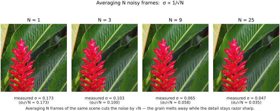
Why does it work, and how fast? This is worth doing carefully once, because the same statistics underlie every denoiser in the chapter. Model a single pixel's measurement as a random variable $X$ with mean $\mu$ (the true value we want) and variance $\sigma^2$ (the noise power). The $N$ frames give us independent draws $X_1, \dots, X_N$ with the same $\mu$ and $\sigma^2$, and we form their average. Two basic facts about variance do all the work (we borrow them from the probability refresher): scaling a random variable by a constant $k$ scales its variance by $k^2$, and the variance of a sum of independent variables is the sum of their variances. So the average $\bar X = (1/N)\sum_i X_i$ has variance
In words: pull the $1/N$ out front (it squares to $1/N^2$), add up $N$ copies of $\sigma^2$, and you are left with $\sigma^2/N$. The variance of the averaged pixel is $N$ times smaller than that of a single shot. Because the standard deviation — the noise level we actually perceive — is the square root of the variance, the noise drops as $1/\sqrt N$: average four frames to halve the noise, a hundred to cut it tenfold. This is the single most important number in denoising, and the metrics follow it directly — SNR and PSNR climb as the variance falls. It also carries a sobering corollary: beating the noise down by another factor of two costs you four times as many frames. There are sharp diminishing returns to throwing photons at the problem.
To average frames you need not know $\sigma$; to evaluate your denoiser you do. The same burst hands it to you: for each pixel, the spread of its values across the frames is an estimate of $\sigma$. One subtlety — divide the summed squared deviations by $N-1$, not $N$ (the Bessel correction). Using the same samples to estimate both the mean and the variance sneaks in a correlation that biases the variance downward; the $N-1$ exactly undoes it. (A two-flip coin makes it concrete: estimate the variance of a fair coin from two flips and the naive $\div N$ gives $0.125$ on average against a true $0.25$, while $\div(N-1)$ gives $0.25$ — unbiased.) A practical guard: variance estimates occasionally come out at zero for no good reason, so clamp them to a small floor before dividing by them.
There is one catch that turns frame averaging from a thought experiment into the engine of modern phone cameras: the frames must be aligned. Hand-held, the scene shifts by a few pixels between shots, and averaging misaligned frames blurs exactly as badly as a careless spatial filter. The fix is to register the frames first — in the simplest form, brute force: try every small shift within a range and keep the one that minimizes the sum of squared differences between frames (alignment is developed properly in the resampling and burst chapters). This align-and-average loop is the heart of every phone that brightens a dark scene by quietly stacking a dozen frames behind the shutter button — the burst / high-dynamic-range (HDR) pipelines treated under multiple-exposure imaging.
Two subtleties about where denoising sits in the pipeline are worth flagging, because both complicate the tidy affine noise model. First, after a burst merge the noise is no longer affine: averaging $N$ frames scales the variance by $\approx 1/N$, but the robust merge keeps a different number of frames per pixel (fewer where something moved), so the residual noise is spatially varying, and highlight clipping (the sidebar below) skews it off the clean gain·signal + read² line. Second, and more fundamental, is the order of denoising and demosaicking. Denoise the raw mosaic before demosaicking and every pixel still carries the sensor's true, near-affine, independent noise — but you are working on a subsampled, one-color-per-pixel image. Denoise after demosaicking and you have full RGB, but the interpolation has already averaged neighboring pixels together: the noise is now correlated between neighbors and spatially non-uniform — an interpolated pixel is quieter than a measured one, by an amount that varies across the frame — so not all pixels have the same variance. Neither order is clearly right, which is exactly why the strongest modern pipelines do neither first and instead solve demosaicking and denoising jointly, as one reconstruction (Demosaicking and joint reconstruction), reconciling the noise model with the interpolation instead of letting them fight.
This is the truncation big lesson from the noise chapter coming home to roost. Recall that the sensor clamps at zero. In a very dark region the true value sits near the floor, and the noise that would have pushed a reading below zero gets clipped away, so the surviving noise is one-sided and its mean is biased upward. Average many such frames and the dark region converges not to black but to a slightly-too-bright gray (and, symmetrically, clipped highlights converge too dark). Camera makers know this — one classic fix adds a small constant offset to the raw signal so the noise stays symmetric and zero-mean before any averaging. It is a good reminder that "average independent noise away" assumes the noise is actually zero-mean, which the physics does not always grant you for free.
4.15.3 denoising from a single image⧉
Usually you have only one photograph. The moment is gone, the subject moved, or there was never a burst. We can no longer average a pixel with other measurements of itself, so we must find our redundant measurements somewhere inside the single image. The governing observation is simple and powerful: most pixels look a lot like their neighbors. A patch of sky, a cheek, a wall — these are regions where the true signal is nearly constant, so neighboring pixels are very nearly repeated measurements of the same value, each carrying its own independent noise. Average a pixel with its neighbors and you get the same $1/\sqrt N$ benefit as frame averaging, for free, from a single shot.
That is the whole idea, and it immediately explains both the easy wins and the hard problem. In flat regions, neighbors genuinely are samples of the same value, and averaging cleans them up beautifully. But at an edge — the boundary between the dark cake and the bright wall — neighbors are not samples of the same value, and averaging them smears the two sides into a muddy band. Single-image denoising is the long story of building filters that average aggressively inside flat regions and refuse to average across edges. Everything below is a different answer to the one question: which neighbors count as the same value?
4.15.4 Spatial averaging and its limits⧉
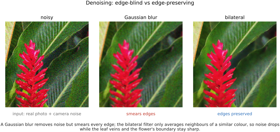
The bluntest neighbor-average is one we already have a name and a tool for: a Gaussian blur (from the convolution chapter). Replace each pixel by a weighted average of a window around it, weighting nearby pixels more than far ones. Since noise is high-frequency — it changes wildly from pixel to pixel — and the true image is mostly low-frequency — it changes slowly — a low-pass filter knocks the noise down and leaves the broad structure standing. And it works: blur a noisy image and the grain is mostly gone (Figure 4.15.2, center).
It is also, of course, blurry. A Gaussian filter has no idea where the edges are; it averages the cake into the wall as happily as it averages the wall into itself, trading a noisy sharp image for a clean smeared one. This is the central tension of single-image denoising, and it is worth naming as a bias–variance trade-off: a wider filter averages more neighbors, so it cuts noise harder (less variance) but blurs more (more bias — detail systematically lost); a narrower filter keeps detail but leaves noise. With a plain Gaussian you only get to slide along that trade-off, never escape it. A median filter — replace each pixel by the median of its neighborhood rather than the mean — does noticeably better on the same budget, because the median ignores the odd wildly-different neighbor instead of letting it drag the average; it is the cheap first upgrade and is excellent against speckle and salt-and-pepper noise in particular.
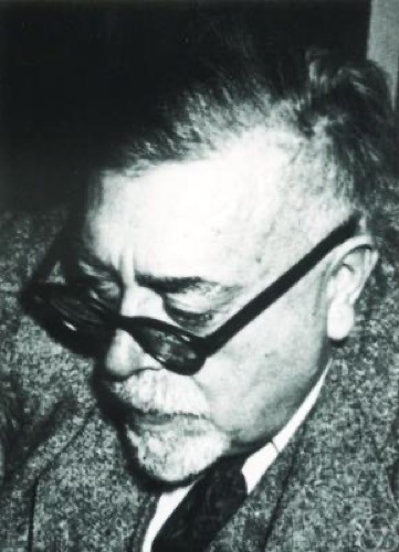 If we insist the denoiser be a single fixed convolution — the same blur everywhere — there is a provably best one, the Wiener filter. Frequency by frequency (think back to Fourier), it keeps a frequency in proportion to how much of it is signal rather than noise: where the true image has strong content it passes through, where the spectrum is mostly noise it is attenuated. It is the right answer to the wrong question — "what is the best shift-invariant filter?" — and its very optimality is the proof that we must leave the world of fixed linear filters to do better. A blur that is the same everywhere can never both smooth the wall and keep the edge crisp. The next idea breaks shift-invariance on purpose. Norbert Wiener (1894–1964) — MIT mathematician, founder of cybernetics — derived this optimal filter from his World War II work on anti-aircraft fire control. Portrait: Konrad Jacobs, Oberwolfach, CC BY-SA 2.0 DE, via Wikimedia Commons.
4.15.5 The bilateral filter: averaging by affinity⧉
Here is the fix, and it is one of the most quietly important ideas in the book. A Gaussian blur decides a neighbor's weight from one thing only: how far away it is in space. The problem at an edge is that a spatially-close neighbor on the other side of the edge has a completely different value, and letting it vote pollutes our estimate. So add a second condition. Weight a neighbor by two factors: how close it is in space, and how close it is in value. A neighbor that is nearby and a similar color gets a strong vote; a neighbor that is nearby but very different in color, because it lies across an edge, gets almost no vote at all. Edges are preserved automatically, because the filter simply declines to average across them. This is the bilateral filter (Tomasi & Manduchi 1998), introduced for exactly this purpose; we build only the intuition here and develop it fully in the edge-preserving chapter.
Concretely, the spatial Gaussian $f$ (a function of position difference, the familiar one) is multiplied by a second range Gaussian $g$ (a function of the value difference between the center pixel $I(p)$ and the neighbor $I(q)$):
In words: for each output pixel $p$, sweep over neighbors $q$; give each a weight that is the spatial closeness $f(p-q)$ times the value closeness $g(I(p)-I(q))$; take the weighted average; and divide by $k(p)$, the sum of those weights. Two things are worth flagging. First, the normalizer $k(p)$ must be recomputed for every pixel, because — unlike a convolution — the weights depend on the local content and so differ at every location. That makes the bilateral filter non-linear and not a shift-invariant convolution; you cannot reuse your convolution code, and you should recompute the range weights $g$ for each pair of values (the spatial $f$ you may still tabulate and truncate at a few $\sigma$). Second, for a color image the "value difference" is a distance in color space — typically the 3-D distance in RGB — so the affinity reflects the full color, not just brightness.
The move that makes the bilateral filter work recurs throughout the book, so name it. Use the color / intensity difference between two pixels as a measure of how much they "belong together" — their affinity. Pixels with high affinity are treated as measurements of the same underlying thing and get averaged; pixels with low affinity (across an edge) are kept apart. The bilateral's range weight $g$ is the first instance of an affinity: a similarity computed from a value difference. Once you see denoising this way, the question "which neighbors count as the same value?" has a clean answer — the ones with high affinity — and the same affinity idea will go on to drive edge-aware tone mapping (the halo fix), edge-aware selections, joint / cross filtering, the bilateral grid, the guided filter, non-local means, colorization, matting and segmentation. We register the lesson here, in denoising, where it first earns its keep; the full edge-preserving treatment — the family of methods and the optimization form — is the subject of the EDGES MATTER part. Edge-preserving is affinity.
A good way to feel the filter — and to debug an implementation — is to push its range parameter to the extremes (Tomasi & Manduchi's own check). Make the range Gaussian very wide, so every value difference counts as "similar," and the value condition stops mattering: the bilateral filter degenerates into a plain Gaussian blur. Make it very narrow, so only near-identical values count, and it refuses to average across even faint differences, leaving edges — and, unfortunately, much of the noise near them — untouched. The useful regime is in between, and the right width is set by the noise level: tell the filter to treat differences up to about $\sigma$ as "the same," and it will smooth the noise while respecting any real edge that exceeds it. A half-black / half-white test image, with a little noise added, makes all of this visible at a glance.
4.15.6 Denoising in the pyramid: coring⧉
A different and very practical single-image denoiser lives in the wavelet / Laplacian pyramid. On natural images the band-pass (detail) coefficients are sparse: a few large coefficients carry the real edges and texture, while a sea of small ones is mostly noise. Coring simply attenuates the small coefficients (zero them, or soft-shrink them toward zero) and keeps the large ones, then reconstructs — flat regions smooth out while edges stay crisp (the denoised before/after sits beside the coring curve in the pyramids chapter, the figure). It is cheap, it respects edges — the large coefficients that are the edges survive untouched — and the affinity here is the simplest yet: "is this detail coefficient big enough to be real?"
The reason coring is still in shipping pipelines decades after fancier methods arrived is that it is finely controllable. Because the image has been split into bands by scale (and, in a steerable or wavelet decomposition, by orientation), you get a separate threshold knob per band: denoise the noisy fine scales hard, leave the coarse structure alone, hit a noisy orientation harder than a clean one, and choose hard thresholding (crisp, keeps contrast, can ring) versus soft shrinkage (smoother, slightly dulls edges) independently at each level. That band-by-band, scale-by-scale tunability is exactly the control a single black-box denoiser does not expose, and it is why a tuner who needs to trade detail against grain at one specific frequency reaches for the pyramid. The statistically principled version models the coefficients' heavy-tailed distributions explicitly — Simoncelli's Bayesian least-squares Gaussian-scale-mixture (BLS-GSM) estimator Portilla et al. 2003 (BLS-GSM) shrinks each coefficient by the amount its neighborhood says is optimal — and for years it was among the strongest non-learned denoisers.
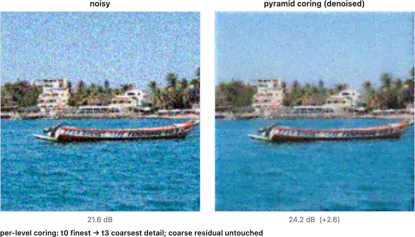
t0 on the finest (noisiest) band down to t3 on the coarsest. The PSNR against the clean original keeps you grounded. The lesson the sliders teach by hand: the finest band carries almost all the noise, so its threshold wants to be high; the coarse bands carry mostly real structure and very little noise, so their thresholds want to be low or zero — turn them up and you start eating edges, and the PSNR drops below the noisy input. That is the whole art of coring in four numbers.The current state of the art is learned: train a neural network (typically a U-Net) on pairs of noisy and clean images and let it discover, from data, both the structure of natural images and the structure of the noise. These now beat the classical methods comfortably, and they shade into generative priors — a network that has learned what clean images look like can hallucinate plausible detail where the noise destroyed it, for better (stunning low-light results) or worse (invented detail that was never there). The link runs deep: diffusion models — the engines behind modern image generators like Stable Diffusion — are trained as denoisers, repeatedly removing a little noise, and a strong denoiser is a strong prior on natural images. The non-local classics (non-local means, BM3D) and these learned and diffusion-based denoisers are developed in the advanced Denoising chapter of the single-image part; here we only flag that the humble averaging idea, pushed to its limit, becomes the most powerful image priors we have.
4.15.7 Denoise color more than brightness⧉
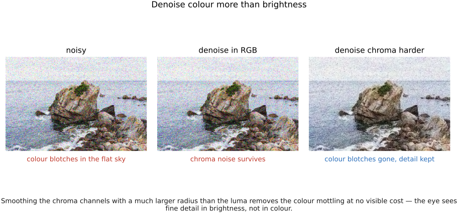
There is a perceptual shortcut that every real denoiser exploits, and it follows straight from how our eyes work. The visual system has much coarser spatial acuity for color than for brightness — we see fine detail in luminance but only blurry, low-frequency color (the same fact that lets the joint photographic experts group (JPEG) format subsample chroma, and that shaped the Bayer mosaic). Noise has both a luminance component (light/dark speckle) and a chrominance component (the blotchy red/green/blue mottling you see in dark areas), and the chrominance noise is both the uglier of the two and the one we can attack hardest without anyone noticing — because we cannot see fine color detail anyway, there is no fine color detail to protect.
So a good denoiser does not work in RGB. It splits the image into a luminance channel and two chrominance channels (a YUV-like space) and denoises them differently: a gentle filter on luminance, where real detail lives and over-smoothing would be obvious, and a much more aggressive one on chrominance — a far larger spatial radius — where heavy smoothing removes the color blotches at no perceptible cost. Run a bilateral filter in YUV with a big spatial $\sigma$ on the chroma channels and the color mottling vanishes while the image stays crisp; the same filter in RGB has to compromise on every channel at once and leaves visible chroma noise behind (Figure 4.15.4). Spend your smoothing budget where the eye won't miss the detail — this is the recurring theme that ties denoising back to human perception.
4.15.8 noise estimation⧉
Every filter above needs to know the noise level: the bilateral's range $\sigma$, the coring threshold, the strength of any smoothing all scale with how much noise there is. Get it wrong and you either leave noise behind (too timid) or erase real detail as if it were noise (too aggressive). There are two ways to find it. The clean way is to calibrate: photograph a flat, evenly-lit field at every ISO setting once, measure the noise variance as a function of signal level, and store a per-ISO noise model (recall the affine read + shot form) that the camera looks up at capture time. The other way is to estimate from the image itself — find patches that look flat and read off their standard deviation, or take a high-frequency residual (the image minus its own blur) and measure its level where there is no real detail. Modern pipelines, knowing the ISO from the exchangeable image file format (EXIF) metadata, mostly use the calibrated model; image-blind estimation is the fallback when you are handed a stray photo with no provenance.
Real noisy/clean smartphone (SIDD) and held-out RAW (DND) denoising benchmarks. <https://www.eecs.yorku.ca/~kamel/sidd/> · <https://noise.visinf.tu-darmstadt.de>. See the Datasets appendix.
With all the filters of this chapter on the table, the most useful thing is to run them against the same noisy image and watch the trade-offs — and the PSNR — move (Figure 4.15.5).
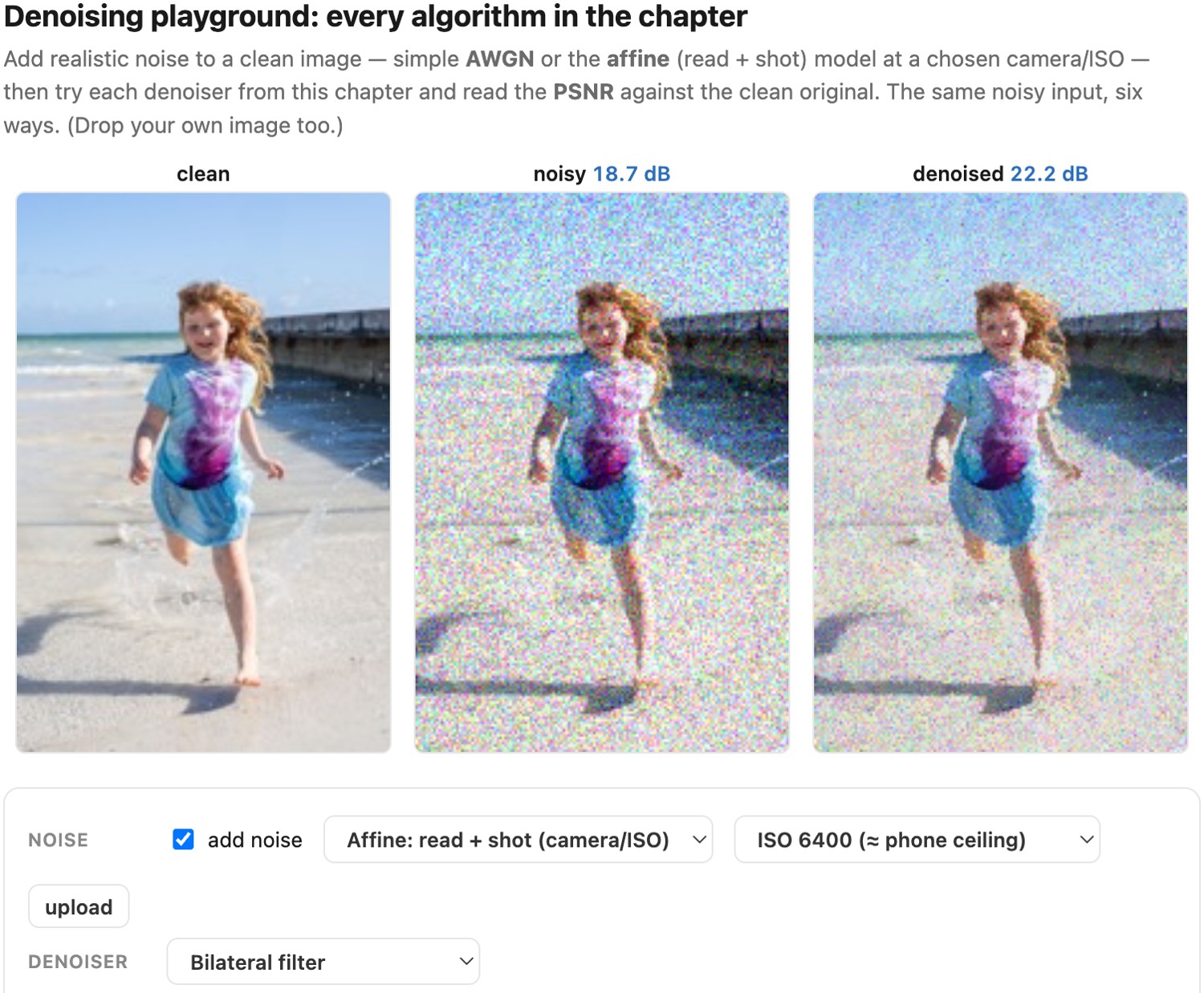
read + shot model at a chosen camera ISO (heaviest grain in the shadows, as the noise chapter predicts) — then try each filter: Gaussian blur, median, bilateral, non-local means, and wavelet / pyramid coring, each with its main parameters exposed. The PSNR against the clean original is printed live for the noisy input and the result, so you can measure what every knob does. The lesson the numbers make concrete: a Gaussian can raise PSNR yet smear edges, while the bilateral and non-local means clean the flats and keep the edges — because they only average pixels that belong together (the affinity idea above). Drop in your own image too.4.15.9 The limits of denoising⧉
It is tempting to think a clever enough denoiser could recover any clean image from any noisy one. It cannot, and it is worth being clear about why. Denoising works by exploiting redundancy — neighbors that agree, patches that recur, frequencies that are mostly signal. Once the noise is strong enough to swamp the local structure, that redundancy is gone: there is no longer a reliable signal in the neighborhood to average toward, and a pixel's true value is genuinely unrecoverable from the data alone. Anat Levin and Boaz Nadler made this precise (Levin & Nadler 2011, extended to finite patches in Levin, Nadler, Durand & Freeman 2012), bounding how much any denoiser — present or future — can recover as a function of the noise level and the statistics of natural images. The bound says there is a floor, and near it the only ways forward are the two we cannot fake: collect more photons (a longer exposure, a bigger sensor, more frames to average) so the signal genuinely rises above the noise, or bring a stronger prior — a model of what real images look like, which is exactly what learned and generative denoisers supply, at the risk of inventing detail that was never measured. There is no free lunch; past the floor, you are either gathering more light or guessing.
One caveat about these bounds: they are stated in terms of mean squared error (an $L_2$ distance to the clean image). That makes the result rigorous, but it also limits what it tells us — an $L_2$-optimal denoiser is not the same as a perceptually optimal one. A result the bound calls "as good as possible" by MSE may still look improvable to the eye, or to a learned perceptual metric (LPIPS and friends, from the Image metrics chapter); and a learned or generative denoiser that hallucinates plausible texture can score worse on $L_2$ while looking far better. So read the Levin–Nadler floor as a sharp statement about information and squared error, not as the last word on perceived quality.
Why should averaging over uncertainty produce something worse than any of the answers it averages? It comes down to convexity, and it is worth holding two complementary perspectives. The first is geometric: the set of natural images is not convex. A convex combination — an average — of two perfectly valid images is, in general, not a valid image; it lands off the natural-image manifold, in the blurry no-man's-land between them (blend a face shifted slightly left with the same face shifted slightly right and you get a ghosted double-face, a member of neither). The minimum-mean-squared-error estimate is exactly such an average over all the clean images consistent with the noisy data, so when those explanations genuinely disagree — a sharp edge that could sit here or a pixel to the side — the $L_2$-optimal answer falls into the gap the manifold curves around, and that gap is where blur and desaturation live. The manifold is messy — non-convex, high-curvature — and averaging across it leaves it. The second perspective is perceptual: the squared-error loss MMSE minimizes treats image space as Euclidean, as though a pixel-wise $L_2$ gap were how we see difference. It is not — human perception is not Euclidean in image space. Two images the same $L_2$ distance from the truth can look worlds apart: a small global shift is perceptually trivial yet $L_2$-enormous, while a little invented-but-wrong texture is perceptually glaring yet $L_2$-tiny. So even setting the manifold aside, the ruler MMSE optimizes is the wrong one, and its "optimal" average is optimal for a notion of distance the eye does not use. The two views reinforce each other — the answer set is geometrically awkward, and the metric we grade it with is perceptually mismatched — which is why the safe average comes out so reliably dull.
Minimizing expected squared error has an exact and revealing answer: the mean of all the outcomes consistent with the data. When the answer is genuinely uncertain — what the denoised patch really looked like, which color was under that gray pixel, what texture filled that hole — the $L_2$-optimal estimate hedges by averaging over all the possibilities, and the average of many sharp, plausible answers is one blurry, desaturated, washed-out answer. This is why $L_2$ denoisers oversmooth, why $L_2$ colourization comes out muddy sepia, why $L_2$ super-resolution is soft: the loss is doing exactly its job, and its job is to play it safe. It is the perceptual flip side of why $L_2$ is so convenient in the first place (Big lesson L4.19, in Image metrics). Escaping the dullness means changing the objective — an adversarial or perceptual loss that rewards a plausible answer over the average one, or a generative model that samples a single sharp outcome instead of averaging them all (the diffusion connection in the sidebar above). And do not then turn around and score the sharper result with the very $L_2$ you abandoned (Big lesson L4.20).
There is an ethical edge to all this that an engineer should see coming. Push denoising too far — especially on skin — and you stop removing noise and start erasing texture: pores, fine lines, the micro-detail that makes skin read as skin. The result is the familiar "plastic" or wax-figure look, and at that point a noise filter has quietly become a beauty filter. The line is genuinely blurry, because skin smoothing, blemish removal, and outright "beautification" are the same operation — suppress the high-frequency variation in regions a face / skin detector has flagged — just dialled further up. Many phones now apply aggressive skin smoothing by default, often without the subject choosing it or even noticing. That should give us pause: it silently imposes a single standard of flawless skin, it is a form of automatic, non-consensual retouching that makes the photograph no longer faithful to the person in front of the lens, and it measurably affects how people — especially the young — see themselves and others. It is worth deciding, when you build a denoiser, where your pipeline draws the line between cleaning an image and editing a face. The book picks this thread up in Human factors, under the candid premise that a photograph was never quite the truth to begin with.
Recap: big lessons of this chapter
The move that makes the bilateral filter work recurs throughout the book, so name it. Use the color / intensity difference between two pixels as a measure of how much they "belong together" — their affinity. Pixels with high affinity are treated as measurements of the same underlying thing and get averaged; pixels with low affinity (across an edge) are kept apart. The bilateral's range weight $g$ is the first instance of an affinity: a similarity computed from a value difference. Once you see denoising this way, the question "which neighbors count as the same value?" has a clean answer — the ones with high affinity — and the same affinity idea will go on to drive edge-aware tone mapping (the halo fix), edge-aware selections, joint / cross filtering, the bilateral grid, the guided filter, non-local means, colorization, matting and segmentation. We register the lesson here, in denoising, where it first earns its keep; the full edge-preserving treatment — the family of methods and the optimization form — is the subject of the EDGES MATTER part. Edge-preserving is affinity.
Minimizing expected squared error has an exact and revealing answer: the mean of all the outcomes consistent with the data. When the answer is genuinely uncertain — what the denoised patch really looked like, which color was under that gray pixel, what texture filled that hole — the $L_2$-optimal estimate hedges by averaging over all the possibilities, and the average of many sharp, plausible answers is one blurry, desaturated, washed-out answer. This is why $L_2$ denoisers oversmooth, why $L_2$ colourization comes out muddy sepia, why $L_2$ super-resolution is soft: the loss is doing exactly its job, and its job is to play it safe. It is the perceptual flip side of why $L_2$ is so convenient in the first place (Big lesson L4.19, in Image metrics). Escaping the dullness means changing the objective — an adversarial or perceptual loss that rewards a plausible answer over the average one, or a generative model that samples a single sharp outcome instead of averaging them all (the diffusion connection in the sidebar above). And do not then turn around and score the sharper result with the very $L_2$ you abandoned (Big lesson L4.20).