4.10 Fourier⧉
An earlier chapter raised a question we now answer. We built blur out of convolution, and we noted that blur is not only something we do to an image but something the world does to us: diffraction, a soft lens, a shaky hand, a missed focus. The natural wish is to run that blur backward — to deblur. That wish organizes this entire chapter. Deblurring is an inverse problem: we are handed the blurred image and asked for the sharp one, which means undoing a convolution. Whether that is even possible, and what it costs, turns out to hinge on a single change of representation: treat the image as a sum of waves instead of a grid of pixels. That viewpoint is the Fourier transform, and reaching it rigorously is most of the work here. The same machinery then powers the very next chapter, on sampling and aliasing — the jaggies, the moiré on a striped shirt, the wagon wheel that spins backward in an old film (Downsampling and aliasing). We cash in the deblurring promise at the very end of this chapter.
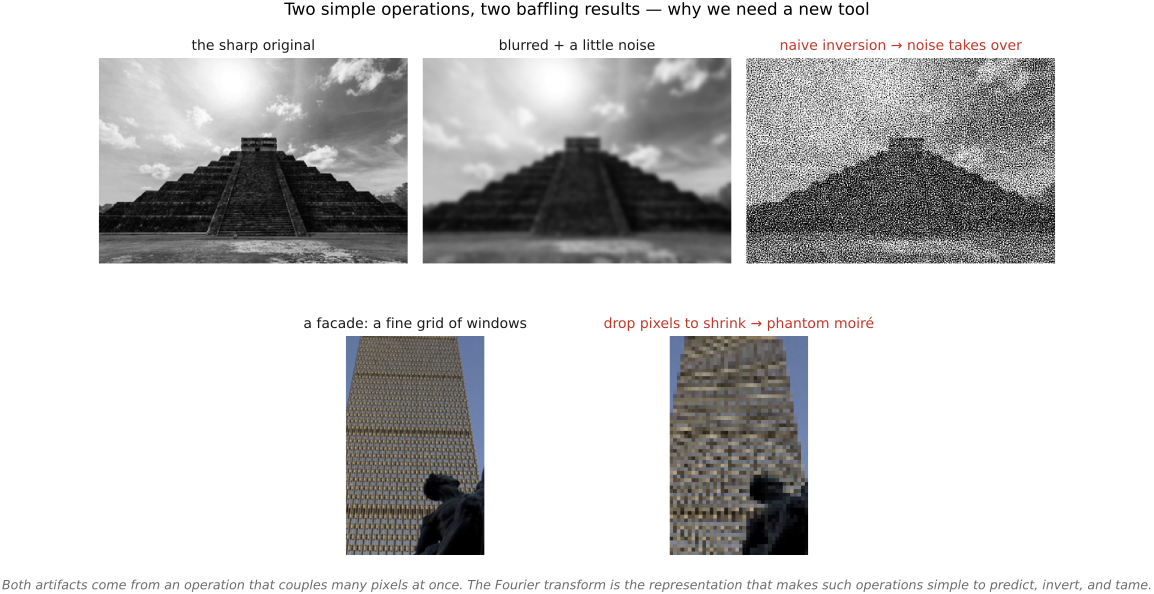
To see why we need new machinery at all, start with two perfectly ordinary operations and the baffling results they can produce (Figure 4.10.1). First, deblurring: take a sharp photo, blur it and add a whisper of noise, then try to undo the blur the obvious way — invert the operation directly. Instead of the sharp original, the result explodes into noise. Second, downsampling: shrink a photo of a building facade by simply keeping every seventh pixel, and bold curved bands appear that are nowhere in the building — phantom moiré. Neither result is a bug; both are doing exactly what we asked. What makes them so hard to reason about is that each operation couples a great many pixels at once — a blur mixes every neighbor into every output, and decimation's fate depends on how the discarded pixels related to the kept ones across the whole image. Staring at the pixels tells us nothing. To understand how these artifacts and patterns emerge — and how to predict, invert, and tame them — we need a different mathematical tool, one in which these many-pixel operations become simple enough to analyze at a glance. That tool is the Fourier transform, and building it is the work of this chapter.
For the very same reason — that it captures blur so cleanly — Fourier is also the standard language for evaluating imaging systems. Because a lens or sensor blurs by convolving with its point-spread function, its quality is naturally read off in the frequency domain as a modulation transfer function (MTF): how much contrast survives at each spatial frequency. MTF curves are how optics are actually specified and resolution is measured (the sidebars below return to this), so the machinery we build here to fight blur is the same machinery the industry uses to measure it.
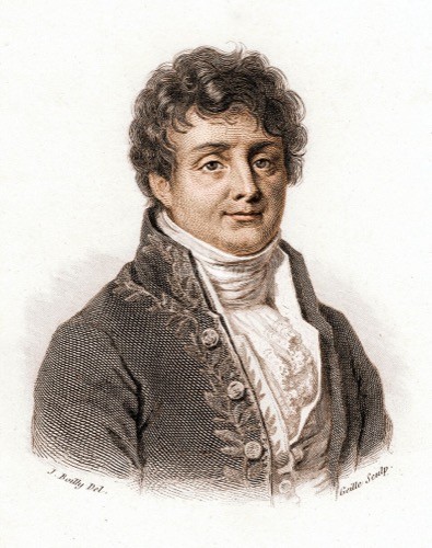 Joseph Fourier (1768–1830) reached his transform not through pure mathematics but through physics — the conduction of heat. In the 1822 Théorie analytique de la chaleur he made the then-scandalous claim that any function, however jagged, can be written as a sum of sines and cosines; contemporaries including Lagrange doubted it, and pinning down exactly when it holds occupied analysts for a century after. The decomposition into frequencies that diagonalizes convolution — the engine of this whole chapter — is his. (Fourier also argued that the atmosphere keeps the Earth warmer than incoming sunlight alone would: the first description of what we now call the greenhouse effect. He was, briefly, Napoleon's governor of Lower Egypt, too.) Portrait: engraving after Julien-Léopold Boilly, early 19th c., public domain (via Wikimedia Commons).
4.10.1 Images as vectors in a high-dimensional space⧉
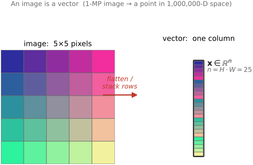
Begin with a reframing that costs nothing and pays for the whole chapter. A grayscale image with $W \times H$ pixels is simply $W\!\cdot\!H$ numbers. Line them up in a fixed order — unroll the grid row by row into one tall column — and the image becomes a single vector, one point in a space with that many dimensions (Figure 1). A one-megapixel image is a single point in a million-dimensional space. The move feels abstract, but it is exactly what lets us bring linear algebra to bear on images, and linear algebra is the sharpest tool we have for the kind of problem we care about. The flattening is sometimes literal — it is, after all, already how the pixels sit in memory and in a machine-learning tensor — and sometimes only conceptual; the image remains, just as validly, a function over pixel coordinates. (For the linear-algebra vocabulary itself — basis, dot product, orthonormality — see the Refreshers appendix; we lean on Strang's Introduction to Linear Algebra as the standard reference.)
Why does the vector view help? Because a great many image operations are linear: brightening scales the vector, adding two exposures adds the vectors, and — the one that matters here — blur is (usually) linear too. Any linear operation on a vector is a matrix. So an optical blur, a motion blur, a Gaussian filter: each is some large matrix $M$ that carries the sharp image $\mathbf{x}$ to the blurred image $\mathbf{y} = M\mathbf{x}$. Deblurring is then, in principle, nothing more dramatic than solving a linear system: invert the matrix, recover $\mathbf{x} = M^{-1}\mathbf{y}$. The entire question of whether we can deblur, and how badly noise will hurt when we try, collapses into a question about a single matrix — and that is a question linear algebra knows how to answer. This dual usefulness, conceptual (a clean language for inverse problems) and practical (we get to call well-tested solvers and libraries), is the reason to adopt the view.
There is one practical worry to dispel immediately. The matrix $M$ for a one-megapixel image is a million by a million — far too large to build, store, or invert directly. The trick, which recurs throughout the book, is that we reason about $M$ without ever forming it. We work out what to do in the abstract language of $M$ and $\mathbf{x}$, then implement it with the cheap image operations that $M$ secretly stands for — a convolution by the blur kernel, a scalar multiply, a dot product of two images. The matrix is the thinking tool; the convolution is the running code. Keeping that separation in mind is what makes the linear-algebra view usable rather than merely elegant.
Linearity is a gift, and we grab it whenever we legitimately can. Sometimes the world genuinely is linear: light adds up, optical blur is a true linear operator. Sometimes we must reformulate to expose a linearity hiding underneath — a multiplicative effect becomes additive in log, perspective becomes linear in homogeneous coordinates (later). Sometimes we simplify a messy reality to a linear model on purpose, because linear tools are so much cheaper and better understood. The caveat for this chapter's physics: images are usually gamma-encoded for storage, while optical and camera-shake blur happen in linear light — so decode to linear before deblurring. The recurring caution of the book holds: idealized linear math rarely fits reality exactly, but its insights almost always survive the mismatch.
4.10.2 why Fourier⧉
Here is the catch with the matrix view. The blur matrix $M$ is enormous, and although each row is actually quite sparse — every output pixel mixes only the handful of inputs under the kernel, so most entries are zero — that local cross-talk is still painful to reason about and, above all, to invert. Undoing the blur means untangling all the overlapping neighborhoods at once, and the inverse $M^{-1}$ is generally not sparse: a clean local operation can have a thoroughly non-local undo. You cannot eyeball a million-by-million matrix and pronounce whether it can be undone. The structure is at least tidy in 1-D: there the convolution matrix is Toeplitz — the same kernel sliding down every row, constant along each diagonal — clean enough to draw. In 2-D that tidiness fragments: once you flatten the grid into a vector, the matrix becomes a block-of-Toeplitz-blocks, far messier to picture even though it is doing the very same local averaging. That is one more reason to change basis rather than wrestle the matrix directly.
There is, however, one species of matrix that is trivial to understand and trivial to invert: a diagonal matrix. A diagonal matrix has no cross-talk: each input coordinate is multiplied by its own scalar, independently of every other. Inverting it is then embarrassingly easy: divide each coordinate by that scalar. The entire difficulty of inversion shrinks to one question per coordinate — how close is that scalar to zero? — because dividing by a near-zero number is where all the trouble lives.
So the goal is clear: we would love the blur matrix to be diagonal. In the pixel representation it is nowhere close. But — and this is the pivot of the chapter — we are free to change how we represent the image, to describe it in a different basis, and a linear operator that looks coupled and hard to invert in one basis can look perfectly diagonal in another. The basis that diagonalizes convolution is precisely the Fourier transform. Change to the Fourier representation and blur stops being a million-dimensional tangle and becomes, instead, a separate scalar multiplication on each frequency — exactly the diagonal case we wished for. (One caveat, which we keep flagging: this exact diagonalization assumes the image is cyclic — that it wraps around at its edges like a torus. Real images do not, so the borders misbehave; the insight survives anyway, which is why we lean on it as an analysis tool more than a literal implementation.)
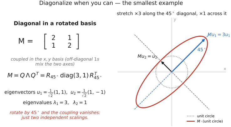
Express a linear operator in a basis where it becomes diagonal. A coupled, hard-to-invert operation in one representation can be a list of independent scalar multiplications in another — and scalars are trivial to understand, compose, and invert. Fourier diagonalizes convolution, turning a blur into per-frequency multiplication. This is not a one-off trick: it is the single most reusable move in applied linear algebra, and it returns for differential equations (the heat equation, below), for principal components, and for nearly every inverse problem in this book. The idea is already visible in the smallest possible case — a $2\times2$ matrix (Figure 4.10.3).
And there is a bonus that makes Fourier feel less like a computational convenience and more like the right language for images. We have already met spatial frequency once, back in perception: the contrast sensitivity function (CSF) describes the eye's sensitivity as a function of how fine or coarse a pattern is — its spatial frequency (see Human perception → Spatial vision / CSF). The visual system is, to a first approximation, organized by frequency. So the Fourier view matches both the mathematics of convolution and the structure of human vision, which is why frequency keeps reappearing — in JPEG compression, in image-quality metrics, in tone mapping. When two unrelated considerations point at the same representation, that representation is usually worth learning.
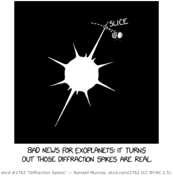
Because light is a wave, wave optics is naturally a story about sines and cosines — so Fourier analysis is usually the right language for it. The vivid everyday case: the star pattern thrown around a bright light when the lens is stopped down is, almost exactly, the Fourier transform of the aperture (its squared magnitude). A round opening gives the Airy disc and rings; a polygonal iris gives a sunstar whose every spike is the Fourier transform of one straight blade-edge — a perpendicular line of ripples — so the star reads out the shape of the diaphragm. The optics performs the transform for free, no FFT required; it is the same physics that makes a small aperture diffract (blur) more, and it returns as the lens's MTF (the transform of its PSF) in the OPTICS part.

4.10.3 Definition: one coefficient per wave⧉
Here is the transform itself, in words first. Instead of describing an image by one value per pixel, the Fourier transform describes it by one coefficient per sine wave. We fix a family of sinusoidal patterns — waves of every frequency that fit in the image — and ask, for each one, how much of that wave is present? The list of answers is the Fourier transform $\hat I$ of the image, and because the operation is perfectly reversible, that list carries exactly the same information as the original pixels: it is the same image, written in a different alphabet.
For an $N$-sample one-dimensional signal the recipe is a sum — one output coefficient $\hat I(u)$ for each frequency index $u$. This is the discrete Fourier transform (DFT):
Read it back in words: to find how much of frequency $u$ the signal holds, slide a wave of that frequency across the signal, multiply point by point, and add up — a dot product between the signal and that wave. The complex exponential $e^{-2\pi i\,ux/N}$ is just a compact way to carry a cosine and a sine of frequency $u$ together, by Euler's formula
so the real part of $\hat I(u)$ measures the cosine content and the imaginary part the sine content. Why carry both? Because a single frequency can appear at any phase — shifted left or right — and a cosine and a sine of that frequency together can reproduce a wave of that frequency at any phase and amplitude. One pair, one cosine and one sine, per frequency. (The naive sum costs $O(N^2)$, but the fast Fourier transform (FFT) computes the very same coefficients in $O(N\log N)$ — the algorithm that made Fourier methods practical, and the reason spectral tricks are cheap in code.)
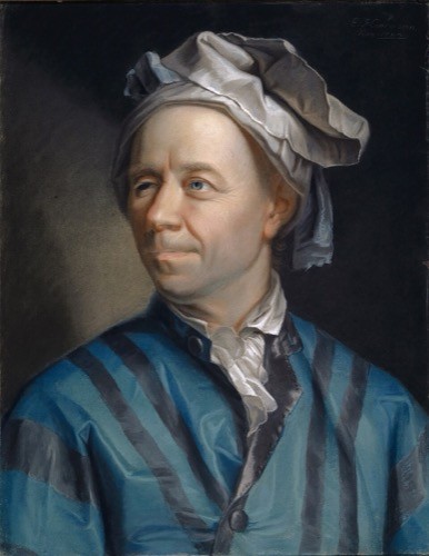 Leonhard Euler (1707–1783) was the most prolific mathematician who ever lived — he kept publishing for years after going blind, dictating from memory. The formula just above, $e^{i\theta}=\cos\theta+i\sin\theta$, is his, and it is what lets a single complex exponential carry a cosine and a sine together — the bookkeeping that makes the Fourier transform compact. His reach into this book is wide: the Euler–Lagrange equations we set to zero to minimize an energy (optical flow, Poisson blending), and the Eulerian "watch a fixed location" view of motion that names half of Feature tracking and all of Video magnification. Portrait: by Jakob Emanuel Handmann, 1753, public domain (via Wikimedia Commons).
A warning to carry out of this chapter, because it will bite the first time you compare a formula against code. The transform above is one of many cosmetically different definitions, and they do not agree digit-for-digit. They differ in the form (the compact complex-exponential here versus separate real sine/cosine series); in where the $2\pi$ lives (in the exponent, folded into the frequency variable, or hidden in the normalization); in which transform you mean (the continuous Fourier transform, the Fourier series of a periodic signal, or the discrete DFT used in code); in the normalization (a $1/N$ on the forward transform, a symmetric $1/\sqrt N$ on each side, or none at all); in the sign of the exponent (forward versus backward — who gets the minus); and in angular versus ordinary frequency. Textbooks, signal-processing courses, and NumPy each pick their own combination, so a formula lifted from one source and dropped into another can be off by a factor, a sign, or a $2\pi$ without any error message to warn you. The rule is simple: always check which convention a source uses before you trust its formula. We use the one above throughout, and — reassuringly — the intuition (a dot product against each wave, convolution becoming per-frequency multiplication) survives every convention unchanged (Figure 4.10.6).

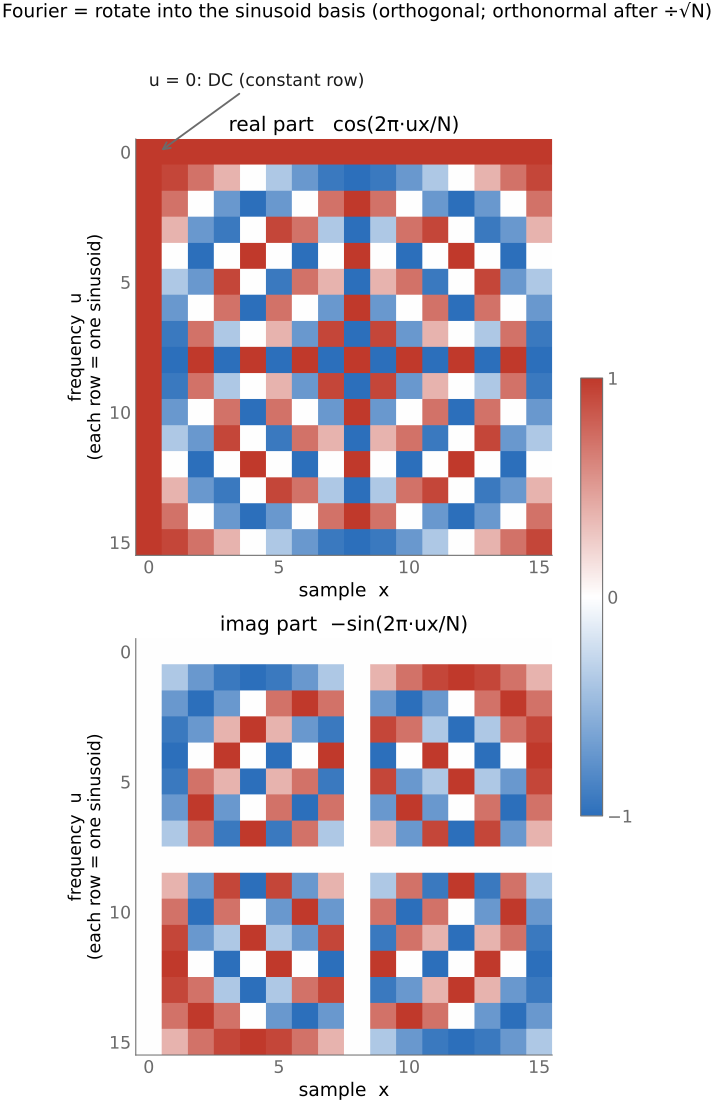
That "dot product against each wave" structure is the main idea of the vector view. The Fourier basis is orthonormal: the waves are mutually perpendicular unit vectors in our high-dimensional space, so finding a coefficient is just projecting the image onto that wave — a dot product, no system to solve. The whole transform is therefore a single matrix multiplication: stack the waves as the rows of a matrix and multiply by the flattened image (Figure 2). And the same orthonormal change of basis that those rows perform is exactly the one that diagonalizes every convolution at once — every linear shift-invariant (LSI) operator. That is the general theorem hiding beneath the chapter: Fourier diagonalizes every linear shift-invariant operator.
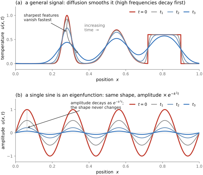
This trick was not invented for images. Jean-Baptiste Joseph Fourier (1768–1830) was trying to solve heat diffusion in a one-dimensional rod with a given initial temperature profile, and the governing equation was a coupled mess. His move, in 1807, was to write the temperature as a sum of cosines — and in that basis the heat equation diagonalizes: each frequency evolves entirely on its own, and a single cosine simply decays exponentially in time ($\propto e^{-k^2 t}$), the highest frequencies fastest, so any profile smooths out. The cosines are the eigenfunctions of the Laplacian (the diffusion operator) — the same reason Fourier diagonalizes our convolutions. Notice what separation of variables has handed us: the two canonical solution families of linear differential equations meeting in one problem — sine waves in space and exponentials in time. The spatial sinusoids set the basis; their amplitudes decay as $e^{-k^2 t}$, the finest ripples dying first, so a general profile melts smooth while a single sine merely fades in place without changing shape (Figure 4). The lesson reaches far past heat: for almost any linear ordinary differential equation (ODE) or partial differential equation (PDE), find the eigenbasis and a coupled system decouples into independent scalar equations whose solutions are plain exponentials ($e^{\lambda t}$) or, for oscillatory systems, sine waves. Diagonalizing is the win.
4.10.4 Sines are the eigenvectors of convolution⧉
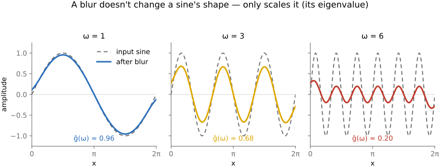
We have asserted that Fourier diagonalizes convolution. Here is the one-line reason, and it is worth seeing because it is the mechanical heart of the chapter. Feed a pure sine wave into any convolution — any blur — and what comes out is the same sine wave: same frequency, only with its amplitude scaled and its phase possibly shifted (Figure 5). The wave is never bent into a different frequency; it is merely turned down (or up) and slid over. In the language of linear algebra, the sine waves are the eigenvectors of convolution, and the per-frequency scale factor is the eigenvalue. Symbolically, convolving a wave $e^{i\omega x}$ by a kernel $g$ just multiplies it by a number $\hat g(\omega)$ that depends only on the frequency:
In words: a blur cannot create or move frequencies, it can only attenuate each one by its own factor. That factor $\hat g(\omega)$ — the eigenvalue at frequency $\omega$ — is exactly the Fourier transform of the kernel. A blur, having a broad smooth kernel, leaves the low frequencies almost untouched ($\hat g \approx 1$) and crushes the high ones toward zero ($\hat g \approx 0$): blur is a low-pass filter, which is just the frequency-domain restatement of "blur removes fine detail."
Because every frequency is scaled independently, the whole convolution, written in the Fourier basis, is diagonal — the eigenvalues $\hat g(\omega)$ sit on the diagonal and nothing else. This is the convolution theorem, and it is the sentence to memorize:
Convolution in space is multiplication in frequency: transform the image and the kernel, multiply their spectra frequency by frequency, transform back. Everything else in this chapter is a consequence of that single identity.
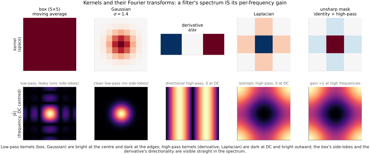
Once you accept that a kernel's Fourier transform is its per-frequency gain, you can read a filter's entire behavior off the shape of $\hat g$ — and conversely recognize a kernel from its spectrum. It is worth building that reflex on the handful of kernels that recur all through image processing (Figure 4.10.10). A box (moving average) is a low-pass, but a leaky one: its transform is a $\text{sinc}$ that dips to zero and rises again in side-lobes, so a box blur lets bands of high frequency leak back through — which is exactly why it makes a poor anti-aliasing filter. A Gaussian is the clean low-pass: a Gaussian transforms to a Gaussian, a smooth monotonic roll-off with no side-lobes. A derivative $\partial/\partial x$ is a directional high-pass whose gain is zero at DC (it annihilates the flat background) and grows with horizontal frequency — it responds to vertical edges. The Laplacian is its isotropic cousin: zero at DC, gain growing outward in every direction. And an unsharp mask (identity plus a high-pass) is the mirror image of a blur — a gain near one at low frequencies that rises above one toward the high ones, boosting detail. Five kernels, five spectra, and in each case the spectrum tells you at a glance what the filter keeps, kills, or amplifies.
4.10.5 The 2-pixel example⧉
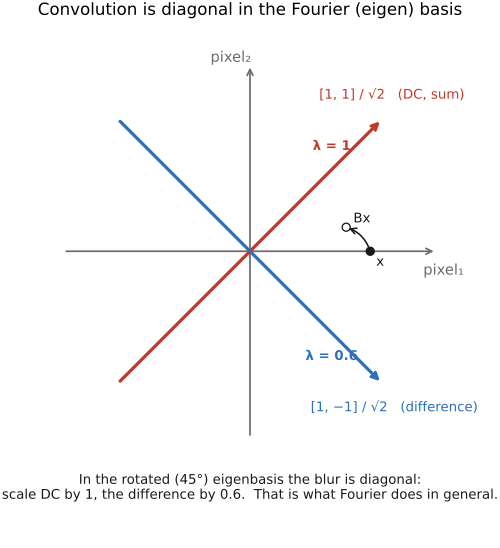
A million dimensions is impossible to picture, so shrink the image to two pixels — a vector in the ordinary 2-D plane, with the two pixel values as its $x$ and $y$ coordinates (Figure 6). Take the simplest blur: each output pixel is $0.8$ of itself plus $0.2$ of its neighbor. As a matrix in the pixel basis this mixes the two coordinates — it is not diagonal; the off-diagonal $0.2$ is the cross-talk.
Now rotate the coordinate axes by 45°, onto the two directions $[1, 1]$ (both pixels equal — the constant, the zero-frequency or direct current (DC) term, borrowing the electrical-engineering name) and $[1, -1]$ (the two pixels opposite — the highest frequency a two-pixel image can carry). That 45° rotation is the Fourier transform for a two-pixel signal. And in these rotated axes the very same blur is diagonal: the constant direction $[1, 1]$ passes through untouched (a flat signal cannot be blurred — eigenvalue $1$), while the oscillating direction $[1, -1]$ is attenuated to $0.6$ (since $0.8 - 0.2 = 0.6$, the high frequency is damped). Two pixels, two frequencies, two independent scale factors — the entire apparatus of the chapter in a picture you could draw on a napkin. Everything that follows is this, scaled up to a million dimensions.
4.10.6 Reading an image's Fourier transform⧉
For a 2-D image the recipe is the same with two frequency indices $(u, v)$ — horizontal and vertical — so the transform is itself an image, the same size as the original, with a value at each frequency. We display it as two pictures: a magnitude (how much of each frequency is present) and a phase (where each wave sits). A handful of properties make these readable.
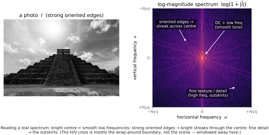
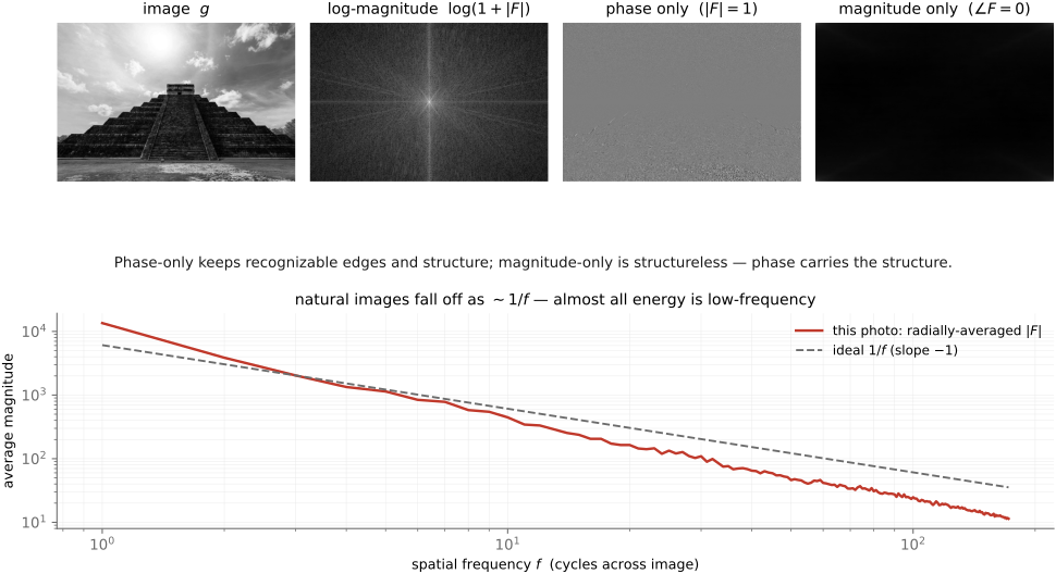
First, a real image has a conjugate-symmetric spectrum: the coefficient at frequency $(u, v)$ is the mirror of the one at $(-u, -v)$, so half the coefficients are redundant and the magnitude image is point-symmetric about its center. The very low frequencies (slow, large-scale variation) sit near the center; the high frequencies (fine detail, sharp edges) sit out toward the corners. Natural images put most of their energy at low frequencies — the world is mostly smooth, with detail concentrated at edges — so a typical magnitude spectrum is bright in the middle and dim at the edges, often with bright streaks where strong oriented structure (a horizon, a picket fence) lives. Set a real photograph beside its log-magnitude spectrum and you can read these correspondences off directly (Figure 7): the bright center is the smooth tone, oriented scene edges show up as bright streaks through the center, and fine texture fills the outskirts. (Beware: the cyclic wrap-around assumption itself injects a cross of horizontal and vertical power, from the discontinuity where the image's left edge meets its right; serious analysis windows the image first to suppress it.)
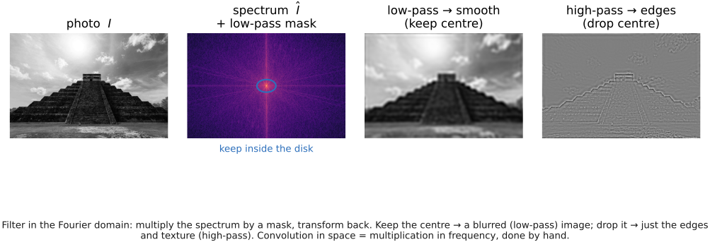
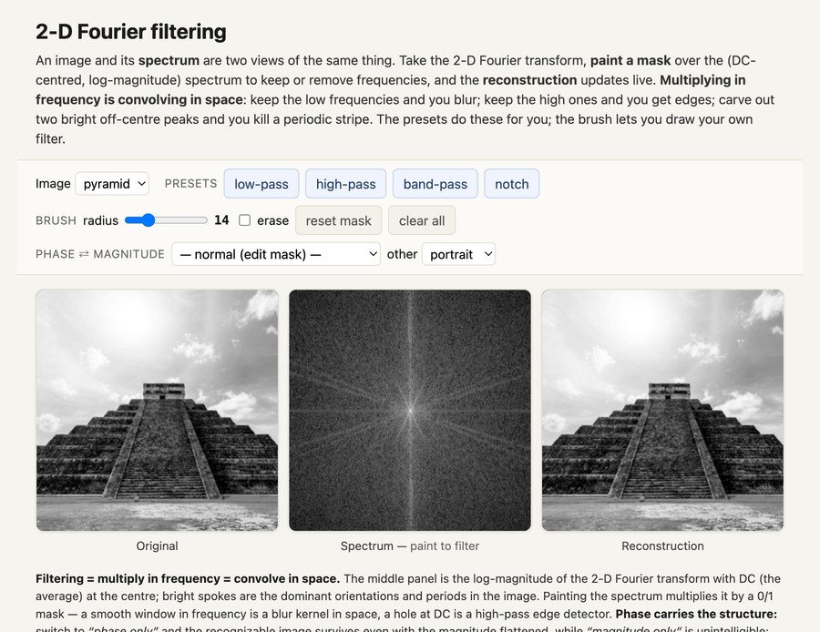
A second reading aid is to manipulate the spectrum and watch what returns. Because filtering is multiplication in frequency, we can low-pass or high-pass a real photo by hand: transform it, multiply the spectrum by a mask — a disk that keeps only the center, or its complement that keeps only the outside — and transform back (Figure 8). Keep the center and the fine detail is gone: a smooth, blurred image, since the detail lived in the high frequencies we deleted. Keep the outside and only the edges and texture survive, the smooth tone subtracted away. This is the convolution theorem turned into an operation you can watch.
This low-pass/high-pass split is so useful that retouchers reinvented it by hand, without ever transforming to the frequency domain. The technique is called frequency separation, and it is a staple of portrait and product editing in Photoshop: blur a duplicate layer to isolate the low frequencies (the smooth tone and color transitions), subtract that from the original to recover the high frequencies (the pores, hairs, and fine texture) on a second layer, and then edit each independently — even out blotchy skin tone or color on the low-frequency layer while leaving pore detail perfectly crisp on the high-frequency layer, or vice versa. It is exactly the two-band decomposition above (a low-pass plus its high-pass complement, which sum back to the original), arrived at pragmatically by photographers who needed to touch tone and texture separately; the major retouching tutorials walk through the layer recipe in detail (Frequency separation (Photoshop retouching technique)).
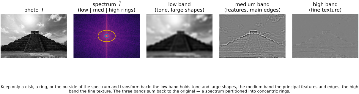
Nothing stops us at two bands. Split the spectrum into three concentric regions — a central disk, a surrounding ring, and the outside — and transform each back on its own, and the image falls apart into a low, a medium, and a high band (Figure 4.10.16). The low band carries the smooth tone and the large-scale shapes; the medium band carries the principal features and edges — the scale at which you actually recognize the subject; the high band carries the fine texture and the sharpest edges, and for a natural photo it holds little energy, which is why it looks faint. Added back together the three bands reconstruct the original exactly, because the rings tile the whole spectrum with no gaps or overlaps. This is the simplest possible multi-band decomposition, and partitioning frequency into rings like this — but done efficiently and at every scale at once — is precisely the idea the Laplacian pyramid will make practical in the next part (Pyramids and wavelets).
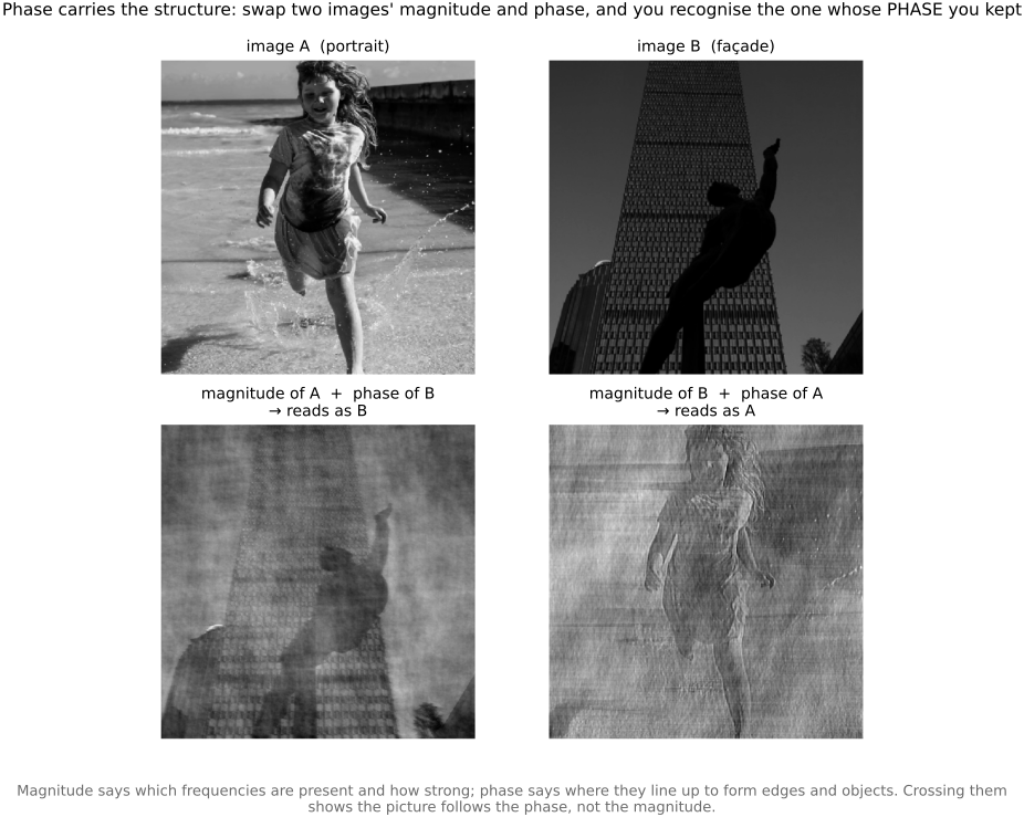
Second, and more surprising: it is the phase, not the magnitude, that carries the structure of a scene. The magnitude reports which frequencies and orientations are present; the phase reports how they line up to form edges and objects. The standard demonstration is to swap them — take the magnitude of image A with the phase of image B — and you recognize the image whose phase you kept, not its magnitude (Figure 9). Phase is where the picture lives.
The cleanest version of this demonstration uses two real photographs and crosses them both ways at once (Figure 4.10.18). Take a portrait, A, and a building, B. Build one image from A's magnitude and B's phase, and another from B's magnitude and A's phase, and inverse-transform each. The first looks like the building, the second like the portrait — every time you recognize the image whose phase you kept, even though its magnitude was thrown away and replaced wholesale. Magnitude is almost a spectator; phase is the picture. (This is also a warning for any pipeline that touches only magnitudes — a magnitude-domain denoiser or compressor that scrambles phase will destroy structure far faster than its numbers suggest.)
A spatial shift, third, shows up as a pure phase ramp — sliding the image over does not change which frequencies are present (the magnitude is identical), it only re-times them (the phase rotates). This is consistent with the eigenvector picture: a shift is a convolution by a shifted impulse, and a convolution can only rescale each frequency by a complex number of magnitude one — a pure rotation, i.e. a phase change.
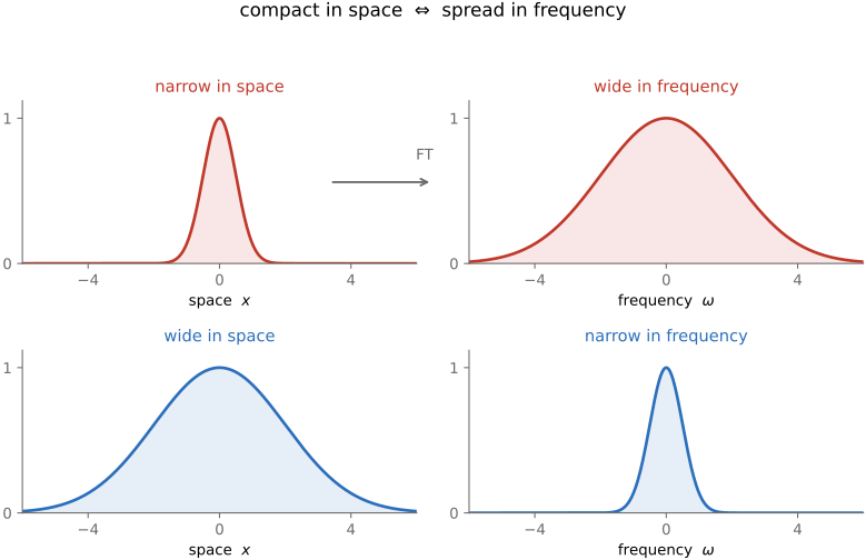
Fourth, the compact-in-space / spread-in-frequency tradeoff. A narrow, sharply localized blob in the image has a wide spectrum, and a wide smooth blob has a narrow one (Figure 10). A Gaussian makes this exact: the narrower the Gaussian in space, the wider its Fourier transform — which is itself a Gaussian. You cannot be compact in both domains at once. This locality-versus-frequency tradeoff is a genuine uncertainty principle, and it is the reason we will later want pyramids and wavelets, which sit halfway between the pixel and Fourier representations to buy some localization in both.
The same language describes a lens. An optical system blurs by its point spread function (PSF) — the little smudge a perfect point of light becomes — and convolving the scene by that PSF is exactly the blur of this chapter. Its Fourier transform, the per-frequency attenuation, is the modulation transfer function (MTF): it reports, for each spatial frequency, how much contrast the lens preserves. A perfect lens would have $\text{MTF} = 1$ everywhere; a real one rolls off toward high frequencies, and diffraction sets a hard ceiling past which no contrast survives — the diffraction limit (see Optics). The MTF is how lenses are actually specified, and it is the frequency-domain face of the PSF — the very low-pass attenuation we will have to fight when we try to deblur.
4.10.7 A small bestiary of transforms⧉
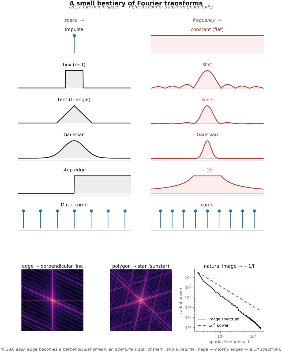
A handful of shapes recur so often that knowing their transforms by sight is most of the working intuition. Each pairing reinforces the space–frequency tradeoff (narrow here = wide there) and connects back to operations we already use (Figure 4.10.20).
- Impulse (delta) ↔ constant. A single bright point contains every frequency in equal measure — a flat spectrum; conversely a constant (DC) is a single spike at zero frequency. This is why a point source probes a system's whole frequency response — the PSF's transform is the MTF.
- Box (rect) ↔ sinc. A hard-edged box of width $w$ transforms to $\operatorname{sinc}(w f)$ — a central lobe with side-lobes that decay only as $1/f$. Wider box → narrower sinc. Those slowly-dying side-lobes are the ringing a hard cutoff causes, in either domain.
- Tent (triangle) ↔ sinc². A triangle is a box convolved with itself, so its transform is the box's squared, $\operatorname{sinc}^2$, whose side-lobes now fall as $1/f^2$ — faster, less ringing. That is exactly why a tent (linear interpolation) is a gentler filter than a box (nearest-neighbor).
- Gaussian ↔ Gaussian. The Gaussian is (up to scale) its own transform: the one shape with no ringing at all in either domain, and a narrow Gaussian ↔ a wide one — the space–frequency tradeoff in its purest form.
- Step edge ↔ ~$1/f$. A sharp step's spectrum falls off as $1/f$ (its derivative is an impulse, flat in frequency; integrating divides by $f$). An edge is "all frequencies, weighted $1/f$."
- Comb ↔ comb. A train of impulses transforms to another train of impulses — the fact behind sampling, in the next chapter.
The last rows tie back to the physics, and to a fact worth carrying everywhere. In 2-D, a straight edge transforms to a line of energy in the frequency plane running perpendicular to the edge — the edge's 1-D $1/f$ profile, smeared along the edge's own direction. A polygon (a stopped-down aperture, say) is just a set of straight edges, so its transform is a star of such perpendicular lines — precisely the diffraction sunstar of L4.9 above, each ray the transform of one blade-edge. And because a natural image is, to a first approximation, a collection of edges at all orientations, each contributing a $1/f$ profile, photographs characteristically have a $1/f$ spectrum: most of their energy at low frequencies, falling off inversely with frequency, with oriented streaks where strong edges line up. That single fact — images are mostly edges, and edges are $1/f$ — explains the shape of nearly every image spectrum you will plot, and underlies why low frequencies dominate, why compression spends most of its bits there, and why natural-image priors are written in terms of sparse gradients.
4.10.8 The fine print: two limitations of Fourier⧉
Before we lean on this machinery any harder, two caveats are worth stating plainly, because the rest of the book keeps bumping into them. Both have surfaced already in passing; here they are named, because each one is the seed of a later idea.
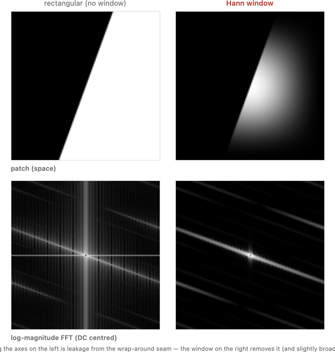
The first is the one we have been flagging since the beginning: the DFT treats the signal as cyclic — periodic. It does not see a finite image with edges; it sees that image tiled to infinity, wrapping around so that whatever runs off the right edge re-enters on the left, and whatever leaves the top returns at the bottom. Where the left edge and the right edge disagree — which, for any real photograph, is essentially everywhere — that wrap-around manufactures a hard artificial discontinuity, and a discontinuity is broadband: it sprays energy across all frequencies. That spurious energy is the boundary leakage that lays a faint cross of horizontal and vertical power over a real spectrum, and it is the ringing that haunts frequency-domain filtering near borders. It is exactly why serious spectral analysis windows the image first — tapering it to zero at the edges so the wrap-around seam vanishes — and exactly the periodic-boundary assumption baked into any FFT-based deblurring solver, which silently inherits this same wrap-around and must be coaxed not to ring at the frame's edge.
The second cuts deeper, and we met its shadow in the space-versus-frequency tradeoff just above. The Fourier basis has infinite, global support: every single coefficient is a wave that spans the entire image, edge to edge. So a Fourier coefficient can tell you which frequencies are present, but it cannot tell you where — there is no spatial localization at all. Move one pixel, or paste a small bright object into one corner, and in principle every coefficient changes, because every global wave must be re-weighted to account for that one local change. This is not a flaw to be patched but a fundamental property of a global basis, and it is precisely what motivates the wavelets and pyramids of the next part: representations that sit halfway between pixels and Fourier, trading a little frequency precision for the ability to say where in the image a given band of detail lives (Pyramids and wavelets). The uncertainty principle we saw with the Gaussian, compact in space or compact in frequency but never both, is the same limitation, seen from the other side.
Fourier diagonalizes convolution beautifully, but at two prices: it treats the signal as cyclic (wrapping at the edges, which real images do not), and its basis waves have infinite, global support (so an idealized frequency operation wants an infinitely wide spatial kernel). Real images are finite and demand compact-support operators. So the insights of Fourier — which frequencies are present, how invertible an operator is, where noise will blow up — are indispensable, but the implementation is almost always a compromise between the Fourier ideal and the reality of finite, non-cyclic images: windowing, padding, truncated kernels. Use Fourier to understand; use compact operators to compute.
4.10.9 Windowing: the price of measuring a real spectrum⧉
The first of those caveats — the cyclic-boundary leakage — is mostly a curiosity when we use Fourier to think, but it becomes a genuine hazard the moment we measure. So it is worth pausing on the one fix, and on what that fix costs.
Recall the mechanism. Take the DFT of an ordinary image patch and the FFT silently assumes the patch tiles periodically: whatever runs off the right edge re-enters on the left. For any real patch those two edges disagree, and that wrap-around jump is a hard, artificial discontinuity. A discontinuity is broadband, and a discontinuity that lives along the patch's straight horizontal and vertical seams sprays its energy along the horizontal and vertical frequency axes — laying down a spurious "+"-shaped cross of power that has nothing to do with the image content. The fix is windowing: before transforming, multiply the patch by a smooth taper — a Hann, Hamming, or Blackman window — that falls to zero at all four borders. With the borders forced to zero there is no longer any seam, the wrap discontinuity vanishes, and the leakage cross with it. The genuine structure — for an angled edge, a clean line of energy running perpendicular to the edge — emerges from under the cross that had been burying it (Figure 4.10.21).
The window is not free, and the tradeoff is the whole story. A taper suppresses the side-lobe leakage, but in exchange it broadens every spectral peak: each sharp spike in the true spectrum is convolved with the window's own transform, so its main lobe widens. And because the taper discards the data near the borders — that is the entire point — it throws away signal and shrinks the effective patch. The two effects trade off directly: a narrower, more aggressive window kills more leakage but blurs frequency resolution and wastes more of the patch, while a gentler window keeps resolution and data but lets more of the cross survive. The named windows are just different points on that curve — Hann, Hamming, and Blackman differ precisely in how they balance main-lobe width against side-lobe height, Blackman buying the lowest side-lobes at the cost of the widest main lobe.
The takeaway, stated plainly: in this book we lean on Fourier almost entirely for conceptual understanding — which frequencies a filter keeps, why deblurring amplifies noise, how sampling replicates a spectrum — and for that work the leakage cross is harmless background that changes none of the conclusions. But anyone who actually measures a spectrum must keep windowing in mind. Measuring a lens's MTF, estimating a sensor's noise power spectrum, detecting a periodic pattern (a sensor-dust fixed-pattern, a halftone screen, a moiré frequency) — in every one of these the leakage cross is a bright artifact sitting exactly on the axes, and an unwindowed measurement will mistake it for real structure. Understand with the rectangular transform; measure with a window.
4.10.10 Application preview: can we deblur, given the blur?⧉
We can finally settle the promise. Suppose we know the blur — the kernel $g$ the optics applied — and we are handed the blurred image; this is non-blind deconvolution (the harder blind case, where the kernel is unknown, waits for a later chapter). The Fourier view makes the question crisp. In the frequency domain, blurring multiplied each frequency of the sharp image by the kernel's eigenvalue: $\hat I_\text{blur} = \hat I_\text{sharp} \cdot \hat g$. To invert, just divide it back out:
This is inverse filtering, and on paper it is perfect. A blur diagonalized into per-frequency multiplications is undone by per-frequency divisions. So why is deblurring not a solved problem?
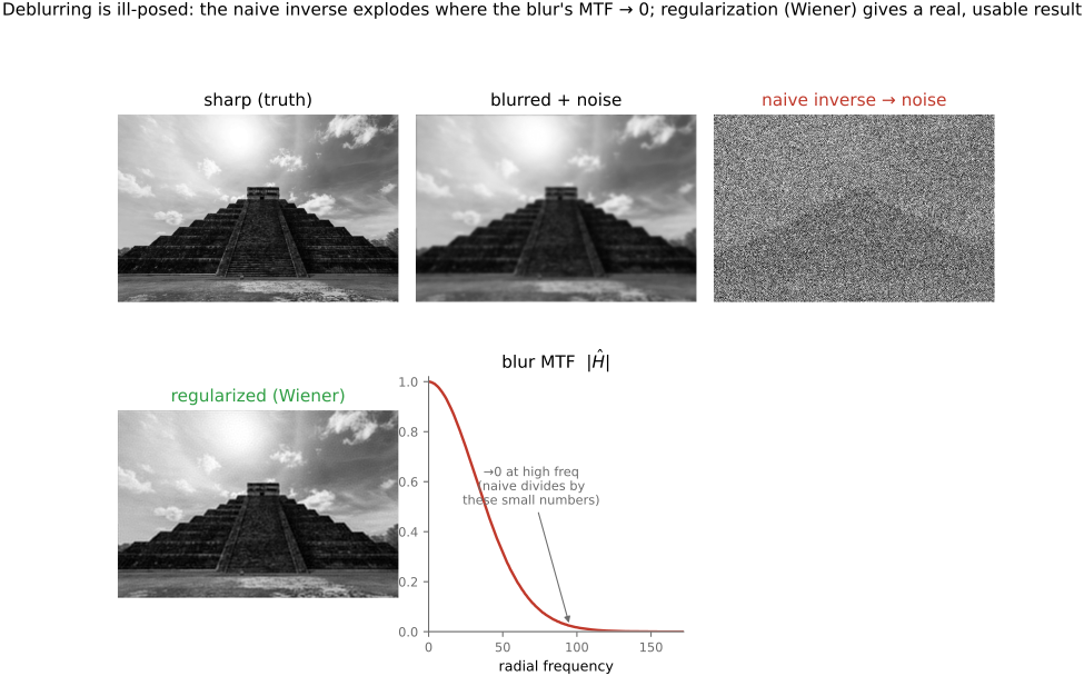
Because of the one number we said decides everything: how close the eigenvalue is to zero. A blur is a low-pass filter, so $\hat g$ is large at low frequencies but tiny — near zero — at exactly the high frequencies the blur destroyed. Dividing by a near-zero number is catastrophic. And real images carry noise: a little random grain the sensor added after the blur, so that what we actually observe is $\hat I_\text{blur} = \hat I_\text{sharp}\cdot\hat g + \hat n$. Divide that through and we get $\hat I_\text{sharp} + \hat n / \hat g$: the genuine signal comes back, but the noise term is divided by $\hat g$ as well. At a high frequency where $\hat g \approx 0.01$ the blur attenuated the signal a hundredfold — yet it never touched the noise, which was added afterward — so dividing by $0.01$ now amplifies that noise a hundredfold. The inverse filter faithfully reconstructs the signal and, in the same stroke, explodes the noise; the result is a sharp-looking image drowned in colorful high-frequency garbage (Figure 15). This is the central difficulty of deblurring, and the Fourier picture diagnoses it exactly: inverse filtering is unstable precisely where the blur was strong.
The way out is to stop dividing blindly. A Wiener filter asks, at each frequency, whether there is enough genuine signal there to be worth recovering: where the blur left healthy signal, divide it back; where the blur crushed the signal below the noise floor, do not bother — leave it attenuated rather than amplify pure noise. It is the optimal linear compromise between sharpness and noise, in effect inverse filtering with a per-frequency safety valve. This regularized view is the foundation; the full treatment — better priors than "minimize noise," gradient-domain and sparsity methods, even designing the lens so its blur has no near-zero frequencies to begin with (coded apertures) — waits for the deblurring chapter. The lesson to carry forward is the diagnosis: deblurring is a division in Fourier, and it amplifies noise wherever the blur's frequency response (its MTF) dips toward zero.
In the Fourier basis a convolution is diagonal: it multiplies each frequency by one number (the kernel's response, the MTF), so undoing it is a per-frequency division. The whole stability question becomes local to each frequency — how near zero is that number? Blur is low-pass, so its response is tiny at exactly the high frequencies it destroyed; the lower a frequency's coefficient, the more its noise is amplified on inversion. That is why naive deblurring fails worst precisely where the blur was strongest, and why a Wiener / regularized filter stops dividing once the signal drops below the noise floor.
Recap: big lessons of this chapter
Express a linear operator in a basis where it becomes diagonal. A coupled, hard-to-invert operation in one representation can be a list of independent scalar multiplications in another — and scalars are trivial to understand, compose, and invert. Fourier diagonalizes convolution, turning a blur into per-frequency multiplication. This is not a one-off trick: it is the single most reusable move in applied linear algebra, and it returns for differential equations (the heat equation, below), for principal components, and for nearly every inverse problem in this book. The idea is already visible in the smallest possible case — a $2\times2$ matrix (Figure 4.10.3).
Because light is a wave, wave optics is naturally a story about sines and cosines — so Fourier analysis is usually the right language for it. The vivid everyday case: the star pattern thrown around a bright light when the lens is stopped down is, almost exactly, the Fourier transform of the aperture (its squared magnitude). A round opening gives the Airy disc and rings; a polygonal iris gives a sunstar whose every spike is the Fourier transform of one straight blade-edge — a perpendicular line of ripples — so the star reads out the shape of the diaphragm. The optics performs the transform for free, no FFT required; it is the same physics that makes a small aperture diffract (blur) more, and it returns as the lens's MTF (the transform of its PSF) in the OPTICS part.
Fourier diagonalizes convolution beautifully, but at two prices: it treats the signal as cyclic (wrapping at the edges, which real images do not), and its basis waves have infinite, global support (so an idealized frequency operation wants an infinitely wide spatial kernel). Real images are finite and demand compact-support operators. So the insights of Fourier — which frequencies are present, how invertible an operator is, where noise will blow up — are indispensable, but the implementation is almost always a compromise between the Fourier ideal and the reality of finite, non-cyclic images: windowing, padding, truncated kernels. Use Fourier to understand; use compact operators to compute.
In the Fourier basis a convolution is diagonal: it multiplies each frequency by one number (the kernel's response, the MTF), so undoing it is a per-frequency division. The whole stability question becomes local to each frequency — how near zero is that number? Blur is low-pass, so its response is tiny at exactly the high frequencies it destroyed; the lower a frequency's coefficient, the more its noise is amplified on inversion. That is why naive deblurring fails worst precisely where the blur was strongest, and why a Wiener / regularized filter stops dividing once the signal drops below the noise floor.