2.5 Measuring and encoding color⧉
The chapter about human color vision provided a liberating observation: because the eye keeps only three projections of a spectrum, a photograph or a screen never has to reproduce the original spectrum — only some light, a metamer, that lands on the same three cone responses. This chapter is the engineering consequence of that single idea. We will see how color is measured against an agreed standard, how the three numbers are packed into a file so that quantization and noise fall where the eye won't notice, how a sensor splits one color into three measurements and a display recombines three into one, and finally how a camera guesses what the light was so it can tell you what the colors are. (Keeping color consistent across devices, the ICC color-management workflow, travels with displays in Displays.) The recurring obstacle behind almost every difficulty is the lesson from the perception chapter that color is non-orthogonal and non-negative, and a new one this chapter contributes about the arithmetic of light itself.
2.5.1 analysis vs synthesis and non-orthogonality⧉
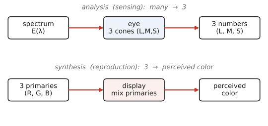
We can split the field of color technology into two mirror-image operations. Analysis is sensing or measuring a color: take an incoming spectrum and project it onto three responses — what the cones do, and what a camera's three color channels do. Synthesis is reproducing a color: take three numbers and build a spectrum that produces them — what a display does by adding a few primaries, what an ink does by subtracting them (Figure 2.5.1). Most devices in this chapter perform one of these two roles (and the full imaging pipeline is analysis at the sensor followed by synthesis at the display, with a great deal of bookkeeping in between).
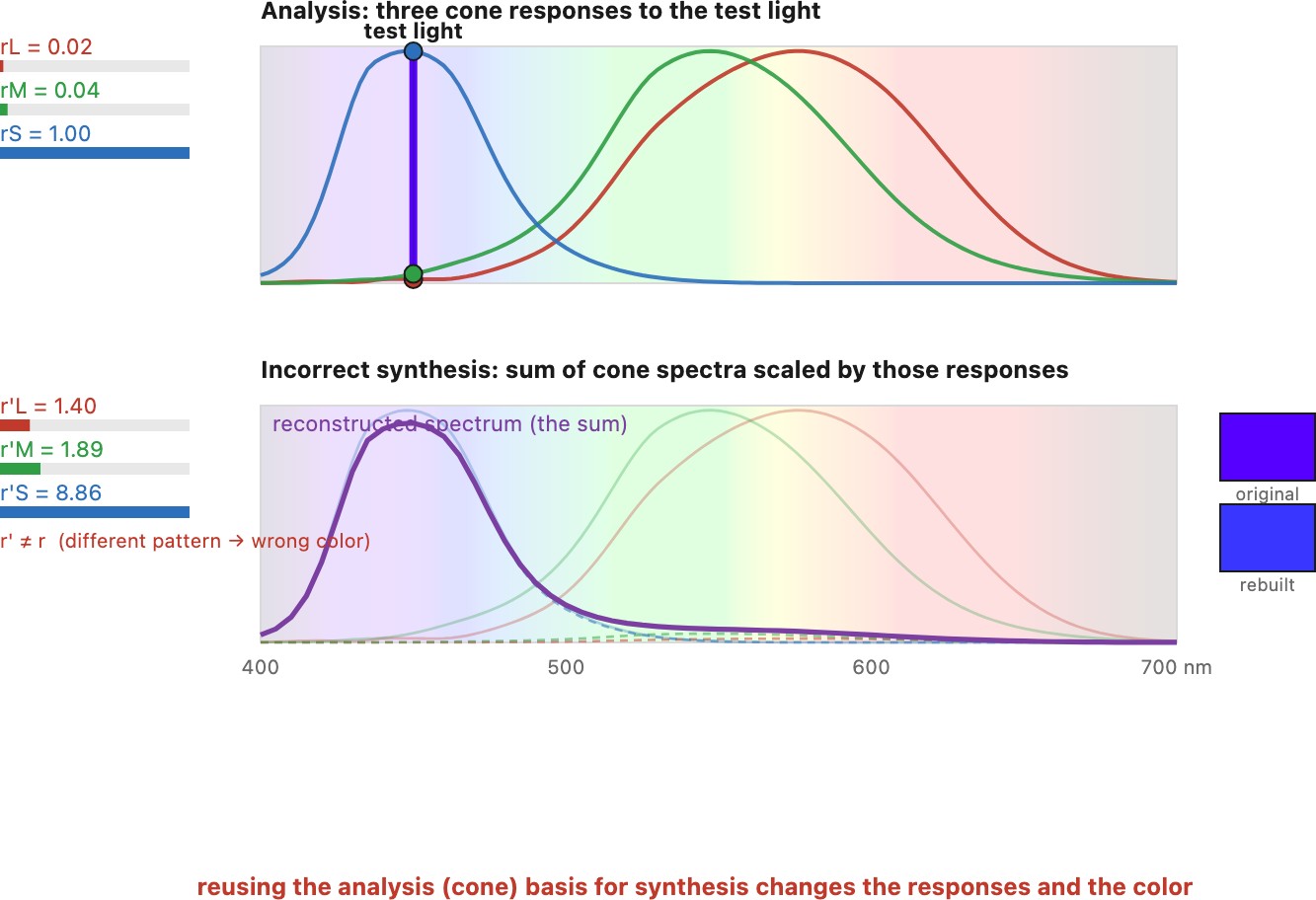
If the cone spectra didn't overlap and the visible spectrum were split into three distinct bins each corresponding to a cone, color technology would be straightforward and we could use the same spectrum for analysis and synthesis. We would measure the power in each bin, pick three primary lights that span one bin each, and scale them according to the 3 measured powers. Unfortunately, the overlap between the three human cone spectra means cross-talk. Imagine using the cone spectra as primary colors and reproducing a color by scaling the LMS spectra according to the response to the same spectra.
Now linear algebra can handle non-orthogonal bases through dual bases. We can still reconstruct any vector in the space if the basis vectors are independent yet non-orthogonal.
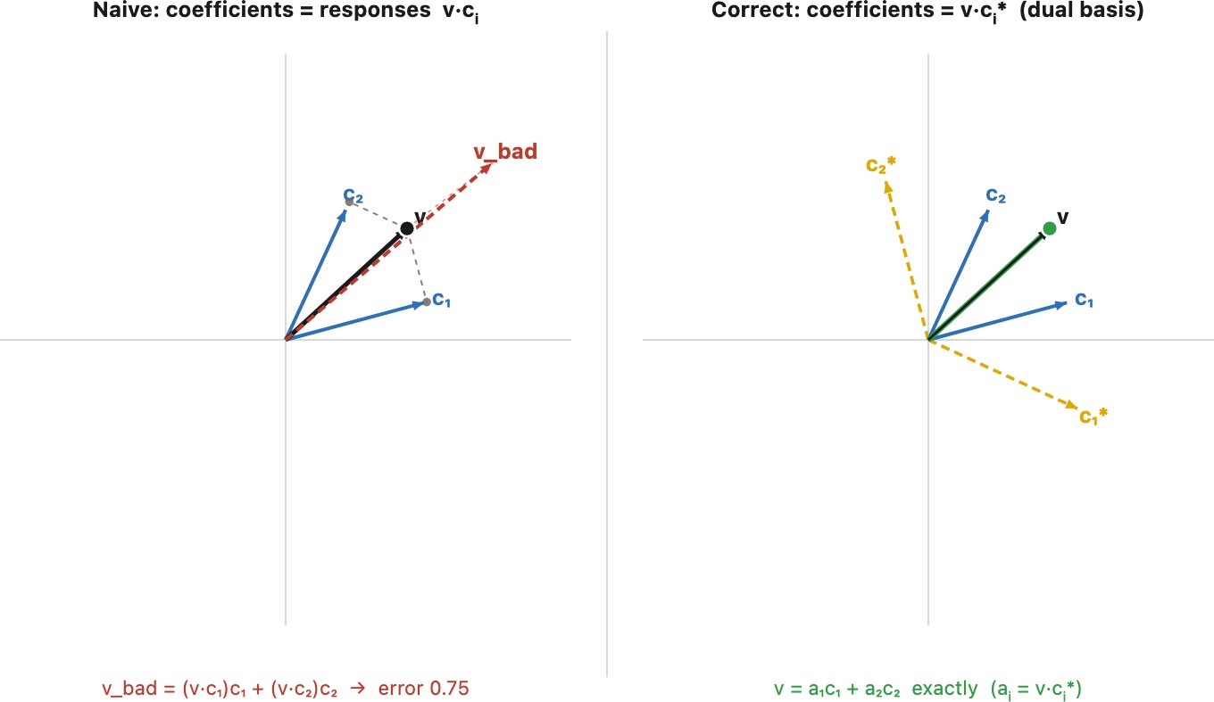
We will mostly be able to leverage linear algebra and , with an important caveat. Dealing with non-orthogonal bases requires combinations that involve negative quantities, and we established that light is always positive. This is why we will not be able to reproduce all possible colors with only three primaries.
It is worth being precise about what problem color reproduction actually solves, because it is not quite the textbook one. In linear algebra, reconstruction means rebuilding a vector exactly as a linear combination of basis vectors, so that the result equals the original. Color reproduction asks for less. We do not need the reproduced spectrum to equal the original spectrum, only to produce the same three cone responses, that is, to be a metamer of it. That is a weaker requirement, a match of projections rather than of whole vectors, and it buys a great deal of freedom: the reproduction primaries can be chosen independently of the analysis (cone) vectors, they can be picked to be physically realizable lights, and the color still comes out right. The dual-basis machinery above is what gets the coefficients right for a given set of primaries; metamerism is what lets us choose those primaries in the first place.
This tension is not a one-time annoyance; it returns at every stage. It is why analysis and synthesis need different sets of vectors (the sensor's spectral responses are not the display's primaries), why no set of real primaries can reach every color, and why white balance is never exact. Keep the two arrows of Figure 2.5.1 in mind: most of this chapter is about doing one of them well, and translating cleanly between the two.
2.5.2 Measuring color⧉
In an ideal world we would measure a color directly against the three cone responses — project the spectrum onto the L, M, S sensitivities (→ Big lesson L2.10) and report those three numbers, and that would be that. But when the CIE set out to standardize color in 1931, nobody could measure the cone spectral sensitivities: the pigments sit in living retinas, far beyond the instruments of the day.
To cut a long story short, they came up with a three-number description of color XYZ that is a linear transformation away from LMS (through a 3x3 matrix) and where one number, Y, corresponds to human perception's notion of brightness. XYZ is the most standard color space, the lingua franca of color, even though almost nobody stores color or images in this format. But all other color spaces are defined with respect to it and the color capabilities of any device are usually expressed in it. Again, in a simpler world, we would simply use the cone responses LMS, but history and inertia made us use XYZ. Furthermore, XYZ has the benefit that Y correlates with our perception of brightness.
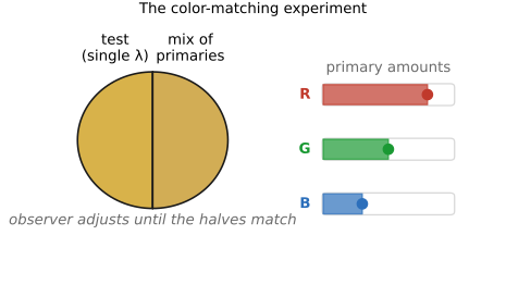
The long story is that they took an indirect route: they defined the analysis of color through its synthesis, leaning on exactly the two facts the perception chapter handed us: metamerism (you need only fool the three cones, not match the spectrum) and linearity (matches add and scale). The plan: measure how each wavelength is perceived by measuring how much of three chosen primaries it takes to reproduce it for a human observer. It is called a color-matching experiment (Figure 2.5.4). An observer looks at a split field: on one side a test light of some spectrum, on the other a mixture of three fixed primary lights whose intensities the observer can dial up and down. The task is to adjust the three primary intensities until the two halves of the field look identical. The three settings that achieve the match are the color's coordinates in that primary system. This works at all only because of metamerism — the observer is not reproducing the test spectrum, just a metamer of it — which is the same good news the perception chapter delivered. Try it yourself on Figure 2. This is a simulation of course since screens usually can't emit arbitrary monochromatic light.
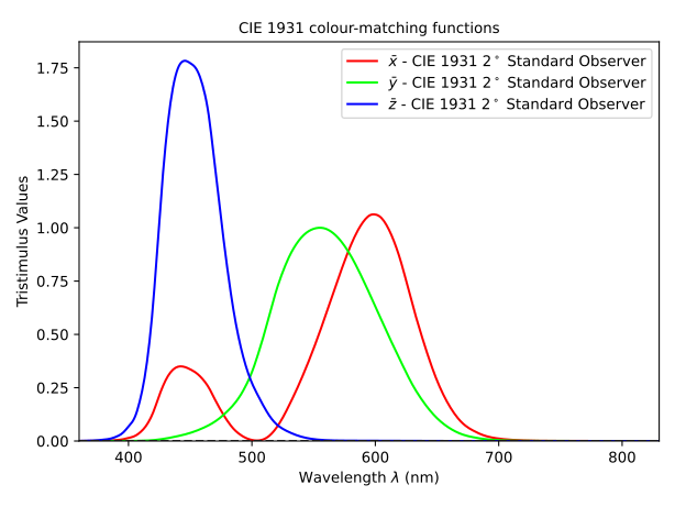
Run this experiment for every monochromatic wavelength across the spectrum and you obtain three curves — the amount of each primary needed to match a unit of light at each wavelength. These are the color-matching functions. Because any spectrum is a sum of monochromatic pieces, and matching is linear, the curves let you predict the match for any spectrum by integration. This is the quantitative form of the trichromatic theory (von Helmholtz, 1859) Helmholtz, Physiological Optics, and the coordinates it produces are the tristimulus values. In 1931 the CIE (Commission Internationale de l'Éclairage, the International Commission on Illumination) standardized one such system for an average human observer, defining the color-matching functions $\bar x(\lambda), \bar y(\lambda), \bar z(\lambda)$ and the tristimulus values
These three integrals are the analysis projection of the previous section, made into an international standard (Figure 2.5.5). The curve $\bar y(\lambda)$ was deliberately chosen to equal the eye's luminance sensitivity, so $Y$ alone is luminance — the perceptual brightness — a convenience we lean on repeatedly below.
And eventually the loop closed. Decades later we could measure the cone sensitivities directly — by microspectrophotometry of single cone outer segments (Bowmaker & Dartnall 1980), suction-electrode recordings, genetics, and careful dichromat psychophysics — culminating in the modern LMS cone fundamentals (Stockman & Sharpe 2000, adopted by the CIE in 2006). Exactly as linearity predicts, the directly-measured cones turned out to be a linear transformation of the 1931 CIE functions, $\mathbf{LMS} = \mathbf{M}\,\mathbf{XYZ}$, with (in the Hunt–Pointer–Estévez normalization)
Frankly, one wishes color had simply been defined in LMS from the start — it is the physically meaningful basis, the one the eye actually uses. But by the time we could measure it, XYZ had half a century of inertia behind it, baked into every standard and instrument. The consolation is that it scarcely matters: XYZ and LMS are one $3\times3$ matrix apart, so the choice is cosmetic. XYZ is only harder to explain, because its primaries are imaginary and its origin is this indirect synthesis route rather than a direct measurement of the cones.
CIE XYZ, the LMS cone responses, and every linear RGB working space (sRGB-linear, Adobe RGB, ProPhoto, a camera's native raw space) are linear transforms of one another — a single $3\times3$ matrix (plus, for a real camera, a fitted approximation). Converting between color spaces is therefore mostly a matrix multiply, and the apparent zoo of color spaces is really one 3-D vector space written in different bases. The non-linear perceptual spaces — CIELAB, the gamma curve — are the deliberate exception, a separate step layered on top (the next sections).
The 24-patch reference chart used to calibrate color and recover illuminants. <https://www.xrite.com/categories/calibration-profiling/colorchecker-classic>. See the Datasets appendix.
LMS (and XYZ) are analysis spectra to measure color. For storing and reproducing color, we usually use color spaces of the RGB family. The most standard RGB version is sRGB, which is given in terms of XYZ by
The linear sRGB primaries are a fixed $3\times3$ matrix times XYZ (both under the D65 white point):
and the inverse recovers XYZ from linear sRGB:
The stored sRGB values are the gamma-encoded versions of these linear primaries (the sRGB transfer function, next sections); the middle row of the second matrix, $(0.2126, 0.7152, 0.0722)$, is exactly the luminance $Y$ as a weighted sum of R, G, B, with green dominant. The negative off-diagonal entries are the familiar signature of a non-orthogonal, positive basis, and any $(R_\text{lin}, G_\text{lin}, B_\text{lin})$ that lands outside $[0,1]$ is a color outside the sRGB gamut (the topic of the next section).
Before we discuss why there is such a large family of RGB standards, we must understand what set of colors can be handles by a given set of primaries, and what information may be lost due to quantization. These are the topics of the next two sections.
2.5.3 Chromaticity diagram⧉
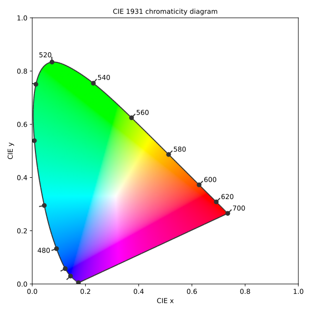
It is convenient to factor brightness out and look only at which color we have, regardless of how bright. Dividing each XYZ tristimulus value by their sum gives the chromaticity coordinates
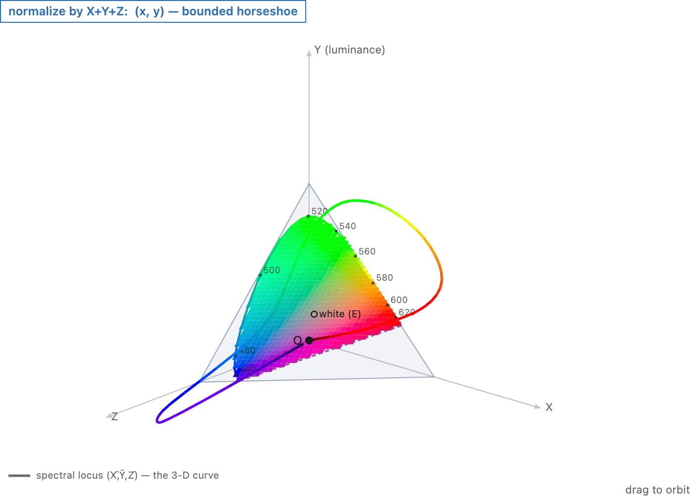
and plotting $(x, y)$ produces the horseshoe-shaped chromaticity diagram (Figure 2.5.6). The author would have preferred CIE divided by $Y$ alone (directly brightness), but dividing by the sum keeps the diagram bounded, as Figure 2.5.7 makes visible in 3-D: normalize by $Y$ alone and the spectral violet and red ends run off to infinity, while dividing by the sum folds every color into a finite region.
Its curved boundary, the spectral locus, is the trail of the pure monochromatic wavelengths; the straight line closing the bottom is the line of purples, which have no single wavelength. Every realizable color lives inside this region, with the neutral white point near the middle. We will hang a great deal on this diagram — gamuts, primaries, white points — so it is worth getting comfortable with it.
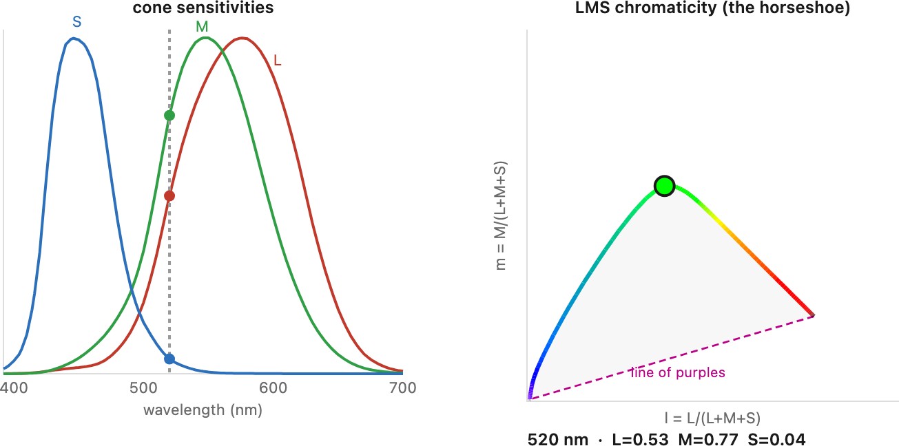
Why is the boundary curved into that horseshoe at all? It all comes from the curves of the cone response spectra (Figure 2.5.8). Because this is really about the cones, it is most faithfully drawn in LMS rather than XYZ; you can sweep a wavelength and watch it ride the rim, on both the cone curves and the LMS horseshoe at once. the XYZ horseshoe is just a linear transformation of this LMS one.
If you want to go deeper, see the geometric explanation Koenderink develops in Color for the Sciences (Koenderink, Color for the Sciences): the set of all physical spectra is an infinite-dimensional cone (spectra are non-negative, and any non-negative combination of spectra is another spectrum), and the eye projects it linearly to the 3-D cone of cone responses. A chromaticity diagram is a flat cross-section of that 3-D cone. The cone's extreme rays are the monochromatic lights — a single wavelength is as "pure" as a stimulus can be — so they trace the cross-section's rim, and the rim is curved for one reason only: it is the image of the cone sensitivity curves themselves. The horseshoe's shape is the shape of the L, M, S curves, seen end-on.
One detail on Figure 2.5.5 deserves a flag because it foreshadows the next several sections: the color-matching curves go negative in places. In the real experiment that means some test colors — highly saturated cyans — cannot be matched by adding the three primaries; the only way to balance the field is to add a primary to the test side instead, which counts as a negative amount. This is the non-negativity wall again. The CIE dodged it by choosing imaginary, "super-saturated" primaries $X, Y, Z$ that lie outside the spectral locus, so that all real colors get non-negative coordinates — at the cost of primaries no lamp can actually emit. That trade (impossible primaries to keep the numbers positive) is exactly the difficulty we confront for real when we try to reproduce color with physical light.
Two more moves finished the 1931 standard, and both are just linear algebra. Because the raw matching functions go negative, the CIE applied a change of basis to a set of imaginary primaries $X, Y, Z$ chosen so that (a) every color-matching function is non-negative, and (b) one coordinate, $Y$, coincides with luminance (the brightness curve $V(\lambda)$). Both conditions are met by a single $3\times3$ matrix applied to the measured curves — trading physical primaries for arithmetic convenience.
2.5.4 Linear vs Gamma vs. log encoding⧉
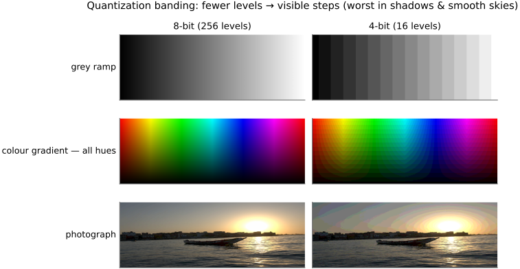
We now have three numbers per pixel; how should we store them as bits? The naïve answer — quantize the linear-light value uniformly — is wrong, and seeing why introduces the most important encoding idea in imaging. The eye's response to light is roughly multiplicative: doubling the light from $1$ to $2$ units looks like the same step as doubling from $100$ to $200$ (the Weber–Fechner law from the perception chapter). A storage scheme that spends equal numbers of code values on equal linear increments therefore wastes precision in the highlights, where the eye cannot tell neighboring levels apart, and starves the shadows, where it can — producing visible banding in dark regions and forcing more bits than necessary (Figure 2.5.9).
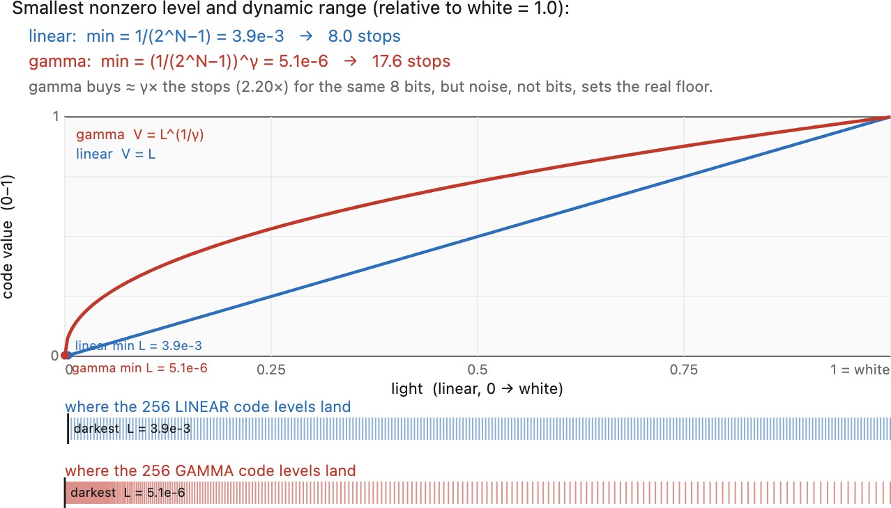
The standard solution is gamma encoding: store a compressed value $V = L^{1/\gamma}$ instead of the linear light $L$, and decode with $L = V^{\gamma}$, where $\gamma \approx 2.2$. The encoding curve devotes more code values to the dark end (where small ratios matter) and fewer to the bright end, matching the eye's sensitivity so that the quantization steps are perceptually even (Figure 2.5.9, left panel — slide γ to watch the code levels redistribute). In practice the sRGB standard uses a piecewise curve — a short linear segment near black, where a pure power law misbehaves, splicing into a $\gamma = 2.4$ power law — but its overall shape is close to $2.2$. Most image files, JPEGs included, hold gamma-encoded values, which is why operations done blindly on pixel numbers (averaging, blurring, resizing) are subtly wrong: they should be done in linear light, a point we return to repeatedly in the image-processing part.
Gamma also changes how much dynamic range a fixed number of bits can represent, at least on paper. Ignore the zero level and ask how far below white the smallest nonzero code sits. With $N$ bits there are $2^N$ levels, so the smallest nonzero step is $1/(2^N-1)$. Stored linearly, that darkest level is $1/(2^N-1)$ of white, about $N$ stops down: eight bits give roughly eight stops. Stored with gamma $\gamma$, the darkest code decodes to $\big(1/(2^N-1)\big)^{\gamma}$, which is about $\gamma\,N$ stops below white, because the encoding curve packs its code values into the shadows. So gamma multiplies the representable range by roughly $\gamma$: the same eight bits now span about $8 \times 2.2 \approx 18$ stops. The interactive figure below lets you set the bit depth and gamma and read off both numbers, alongside the encoding curve and where the code levels actually land.
The catch, and it is a big one, is that this is an upper bound that noise erases. The count of code levels says nothing about whether the darkest ones carry real signal. In a real sensor the floor is set by noise, read noise plus photon shot noise (→ Noise, signal-to-noise ratio and dynamic range), and that floor usually sits well above the darkest representable code. So the extra stops gamma's bit allocation seems to promise are mostly not there: they label levels that noise has already swallowed. Bit depth and encoding decide how finely you label the range; noise decides how much of it you can actually use. It is why "how many stops does $N$ bits give?" is the wrong question and "where is the noise floor?" is the right one.
There is a second, independent reason to gamma-encode, and it is the one that put gamma into television in the first place: noise on the transmission channel. Analog broadcast adds roughly uniform noise to the signal as it travels — but the eye judges brightness by ratio, so a fixed amount of noise is far more visible in the dark parts of the picture than in the bright ones. Gamma-encoding at the camera boosts the dark values before they are sent (the curve gives the shadows more of its range), so the dark signal rides well above the channel's noise floor; the inverse-gamma at the receiver then pulls the highlights — and the noise riding on them, which the eye scarcely notices — back down. The transmission noise is thereby shaped to be perceptually uniform instead of glaring in the shadows. It is the same bit-allocation logic as the quantization argument above — spend your scarce, noisy dynamic range where the eye can see it — but applied to a channel rather than to storage bits, which makes it a textbook case of applied information theory (the communication-channel view of Imaging as an inverse problem). And pleasingly, the CRT's accidental gamma (next sidebar) meant the camera had to pre-encode anyway — so this noise benefit came almost for free.
The specific value $2.2$ is a historical accident worth knowing, because it explains why we still use it. Old cathode-ray tube (CRT) displays had a natural power-law response: screen luminance was proportional to (grid voltage)$^{\gamma}$ with $\gamma \approx 2.2$–$2.5$, a consequence of electron-gun physics (the beam current is a power law in the control-grid voltage). So a CRT automatically decoded a gamma-encoded signal — feed it $V = L^{1/\gamma}$ and the tube emitted $L = V^{\gamma}$, linear light, with no decoding hardware at all. sRGB's $\approx 2.2$ simply codifies that tube curve. The bonus is that this same curve is roughly the inverse of human lightness perception (Weber–Fechner), so it also puts the code levels where the eye is sensitive. That is why we kept gamma after CRTs vanished: a modern liquid-crystal display (LCD) or organic light-emitting diode (OLED) panel emulates the old tube curve purely for compatibility, even though its physics no longer demands it.
Most encodings cluster around a display gamma of ≈ 2.2: sRGB (the web; a piecewise curve whose power segment is $1/2.4$ but whose overall shape is $\approx 2.2$), Rec. 709 / Rec. 1886 (HDTV), and Adobe RGB (1998) all sit there. The exception worth knowing is ProPhoto RGB (ROMM RGB) — the very wide-gamut working space used for high-end raw editing — which encodes with gamma 1.8 (plus a small linear toe near black, like sRGB). A gentler $1.8$ spends relatively more code values in the highlights, which suits a wide-gamut editing space carrying plenty of bit depth. Old Apple/Macintosh displays also used 1.8 for years, which is why files from that era can look wrong when mis-tagged. The practical rule: 2.2 is the safe default, but a gamma number is meaningless without its color space — decode a ProPhoto ($1.8$) value as if it were sRGB ($2.2$), or the reverse, and the result is visibly off (milky, or too contrasty). This is the encoding-as-a-type-system point again: store the curve with the pixels.
The word gamma comes from photography, where it means something related but distinct. Film's response is its characteristic curve (the Hurter–Driffield curve): optical density plotted against log exposure, with a toe in the shadows, a straight middle section, and a shoulder in the highlights. Film gamma is the slope of that straight portion, $\gamma = \Delta D / \Delta \log H$ — the medium's contrast, set by development (push-processing raises it). So film gamma is a contrast/rendering knob while display gamma is an encoding power law; both are log–log slopes, but they do different jobs. End-to-end system gamma (capture $\times$ display) is deliberately tuned slightly above $1$ (about $1.1$–$1.5$) so that images look right when viewed in a dim surround, which washes out apparent contrast.
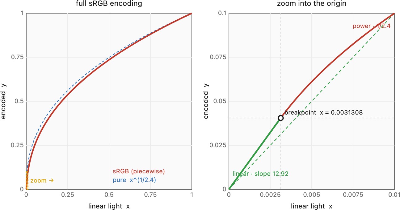
The sRGB transfer curve that every web image lives in is piecewise: a short linear toe near black, $V = 12.92\,L$ for $L \le 0.0031308$, splicing into a power segment $V = 1.055\,L^{1/2.4} - 0.055$ above it. The two pieces are meant to join smoothly at the knee — but the standardized constants ($12.92$, the breakpoint $0.0031308$, the $0.055$ offset, the $1/2.4$ exponent) are rounded and not mutually consistent, so they miss each other: at the breakpoint the linear part gives $\approx 0.04045$ while the power part gives $\approx 0.04059$, a tiny discontinuity of order $10^{-4}$, on top of the slope kink that is there by design. So even the encoding underneath every JPEG is, strictly, not continuous at the join. The lesson is small but practical — real transfer functions are messier than the clean "$\gamma \approx 2.2$" story, so check the actual curve (and its inverse) before you do arithmetic or quantize in that space. (A "corrected" sRGB nudges the breakpoint and scale so the two pieces meet exactly.)
A third common option is log encoding, $V \propto \log L$, which spreads code values evenly across ratios (stops) of light. This is the native language of multiplicative processes, and it is the standard for camera RAW capture in cinema and for high dynamic range (HDR) grading, where the scene spans far more stops than a display can show. The choice among the three encodings is not arbitrary — it follows from the arithmetic of the operation you intend to perform.
Log encoding is, in fact, becoming the standard for video: high-end and now prosumer cameras shoot in named log profiles — S-Log / S-Log3 (Sony), Log-C (ARRI), V-Log (Panasonic), C-Log (Canon), RED Log3G10 — and the ACES (Academy Color Encoding System) pipeline standardizes a log working space (ACEScc / ACEScct). The appeal is that log packs a wide scene dynamic range into limited bits while keeping the grade malleable: a stop becomes a roughly constant code increment, so exposure and contrast moves are uniform across the tonal range. The catch is that the footage looks flat and desaturated straight out of the camera — it is not meant to be viewed, but color-graded down to a display encoding afterward. On the display side the broadcast-HDR transfer functions HLG (hybrid log-gamma) and PQ (perceptual quantizer, SMPTE ST 2084) play the role gamma plays for standard dynamic range. So in modern video the trio increasingly resolves to a single slogan: log for capture, gamma / PQ / HLG for display. The canonical references for all of this — gamma, the luma-versus-luminance distinction below, and video encoding generally — are Charles Poynton's Digital Video and HD: Algorithms and Interfaces Poynton 2012 and his widely-circulated Gamma FAQ and Color FAQ.
Whether light adds or multiplies should dictate how you encode it. Light from independent sources adds (two lamps, the blur of an out-of-focus lens, the accumulation of photons on a sensor) — these are linear operations, and they are correct only on linear-light values, which is why deconvolution, resizing, and physically-based blur must decode the gamma first. Surface reflectance and perceived contrast, on the other hand, multiply (a gray card under twice the light, a filter cutting a fraction of each wavelength) — and a log encoding makes the multiplicative native, turning products into sums. Gamma is the pragmatic compromise: a power law that behaves better than $\log$ near zero (where $\log$ blows up) while still matching perception. Get this wrong — average gamma values, or sharpen in log — and you get milky blurs, wrong colors, and crushed shadows. The same additive-vs-multiplicative split organizes tone mapping, HDR, and point operations later (→ Big Lessons).
(An interactive demo of exactly this — deconvolving a blurred image in the linear vs the gamma-encoded domain — lives in Imaging as an inverse problem, where deconvolution and its conditioning are the subject.)
Finally, a notational trap that this encoding choice creates and that confuses everyone at least once: luma versus luminance. Luminance $Y$ is the true, perceptual brightness — a weighted sum of linear RGB (the CIE $Y$ above). Luma $Y'$ is the same-shaped weighted sum, but computed on the gamma-encoded RGB, as a coding convenience (it is the brightness channel inside the luma-chroma formats YUV (luma Y plus U and V chroma) and YCbCr, and in JPEG). They are not equal, because applying the weights and applying the gamma do not commute. Our convention in this book, matching video, JPEG, and the programming exercises, is the Rec. 601 luma weighting
with green dominating because the eye's brightness sense is mostly green. We will mention the Rec. 709 weights ($0.2126 / 0.7152 / 0.0722$), the high-definition television (HDTV) alternative applied to linear light, where context calls for radiometric correctness.
2.5.5 RGB color spaces⧉
Why is there a zoo of RGB spaces at all, rather than one? The answer is a genuine three-way tension, and every named space is one compromise among the three. First, you want to cover as much of the visible range as possible, a wide gamut, so that saturated reds and greens are representable at all. Second, you have a fixed bit budget: a color is stored in a handful of bits per channel (often 8), and those code values are spread across whatever gamut you chose, so a wider gamut makes each step coarser and invites banding, while a narrower one packs the codes densely where colors actually occur. Coverage and quantization pull against each other: reach for more colors and you quantize each one more crudely; give up reach and you encode the colors you kept more finely. Third, none of this lives in the abstract. A real display can light up only the colors inside its own primaries, and a real sensor or scanner captures only what its filters admit, so a working space also has to be honest about the hardware at each end. The families below are the standard settlements: a capture or editing space (ProPhoto, Rec. 2020) leans toward coverage and pays for it with more bits; a delivery space (sRGB) leans toward efficient, safe encoding on the displays people actually own; and the wider delivery spaces (Display P3, Adobe RGB) sit in between as panels improve. Keep that tension in mind and the list stops looking arbitrary.
With a way to measure color ($XYZ$) and a way to encode it (gamma), we can organize the zoo of named color spaces. The first family is built on RGB. There is no single "RGB" — there are many RGB spaces, differing only in their primaries (which fix the reachable gamut) and their white point (Figure 2.5.14). sRGB / Rec. 709 is the small, safe space of the web and HDTV; Adobe RGB and Display P3 are wider; Rec. 2020 (ultra-high-definition) is wider still; ProPhoto RGB is enormous and used as an editing working space. The crucial fact is that any two of these, or any of them and $XYZ$, are related by a single $3 \times 3$ matrix $M$ — converting between color spaces is one matrix multiply, provided it is done in linear light.
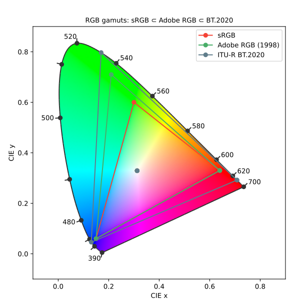
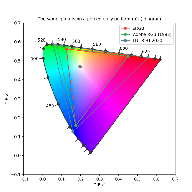
A caution about that diagram before we read too much into the triangle sizes: the $xy$ chromaticity plane is a space for measuring color, not for judging how different two colors look. It stretches the greens enormously and cramps the blues and purples, so neither the relative areas of these gamuts nor the distances between their primaries track perceived difference. Re-plot the identical primaries on a perceptually more uniform diagram, the CIE 1976 UCS ($u'v'$) space, and every triangle changes shape (Figure 2.5.13): the huge green lobe collapses toward its true perceptual size and the blue corner opens up. That $XYZ$ (and its $xy$ projection) is not perceptually uniform is precisely what will force the deliberately non-linear spaces of the next section.
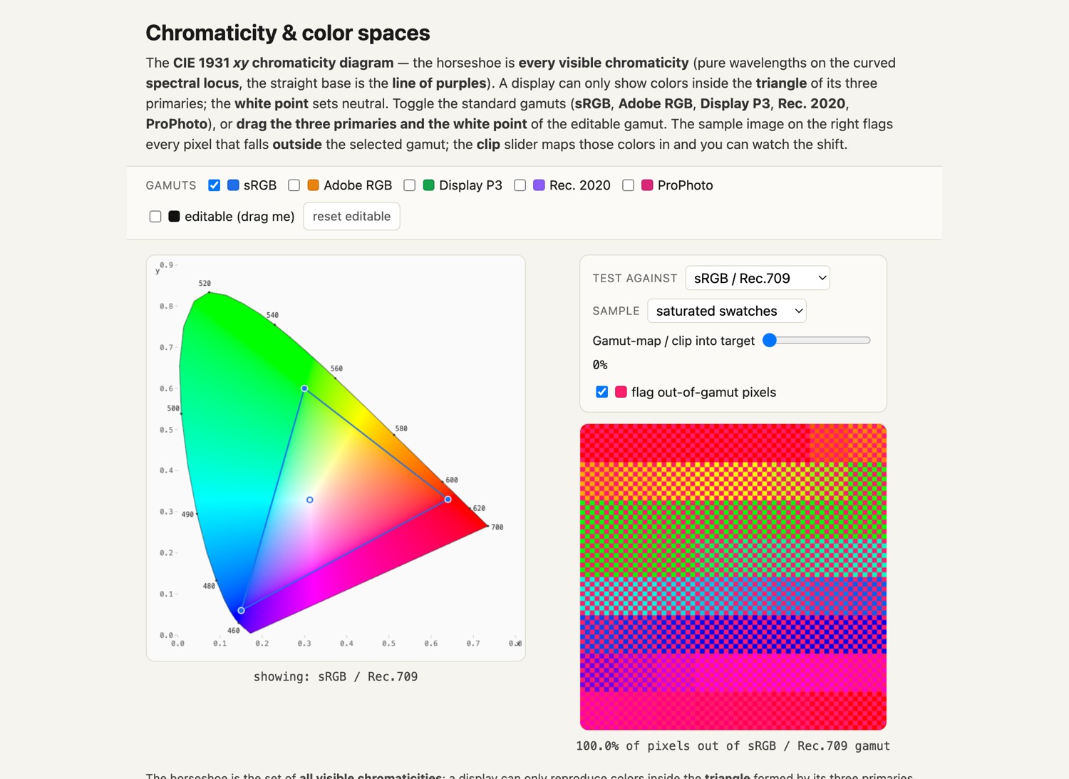
You can take that triangle in your hands in the interactive companion (Figure 2.5.14b — Figure 2.5.14): toggle the standard gamuts on the chromaticity diagram, drag the three primaries and the white point of an editable space and watch its triangle redraw, then test a sample image against any target space — every pixel the target cannot reach lights up, and a slider clips them in so you can see the shift. It makes concrete the chapter's whole point: a display shows only what is inside its primaries' triangle, wider spaces enclose more, and the surplus must be gamut-mapped.
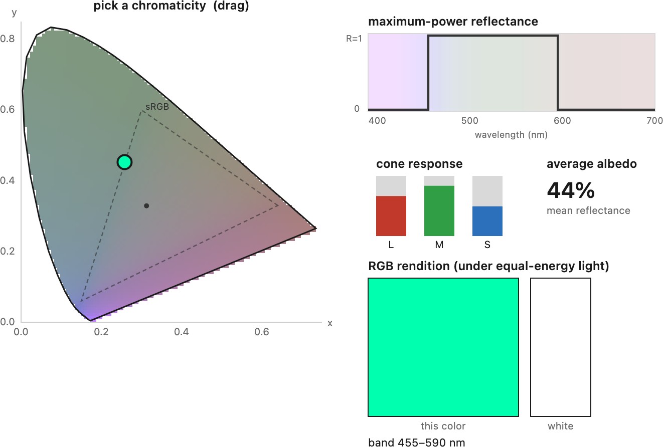
One reassurance about all this gamut anxiety: the colors that fall outside a reasonable RGB gamut are rare in ordinary scenes, and for a physical reason worth understanding. To sit out near the spectral locus, beyond the triangle, a color has to be almost monochromatic, its spectrum concentrated at essentially one wavelength with little power anywhere else. But a surface whose reflectance is that narrow returns only the sliver of the illuminant that happens to fall in its band and absorbs everything else, so it is extremely dark: a near-monochromatic reflectance looks almost black under ordinary broadband light, and only comes alive when it is lit by matching monochromatic light (a laser, a narrow-band LED). Bright and highly saturated colors are, therefore, physically uncommon, which is exactly why a modest gamut like sRGB gets away with as much as it does. The vivid exceptions all involve narrow-band spectra that carry real power rather than reflecting it, saturated LEDs and lasers, some fluorescent dyes, and the iridescent structural colors of beetles and feathers, and those are precisely the cases that push past a display's primaries and demand gamut mapping.
You can watch this trade-off directly in the interactive companion (Figure 2.5.15): pick any chromaticity on the diagram and it shows the brightest physical reflectance that can produce it, the surface that reflects the most light while still landing on that color. Drag toward the white point and the reflectance is a broad band, so the surface is bright; drag out toward the spectral locus and the band collapses to a single wavelength, monochromatic and nearly black. The average albedo falls to almost nothing as you approach the edge, which is the whole reassurance made visual: a saturated color can only be made by throwing most of the light away, so bright-and-saturated surfaces are physically scarce.
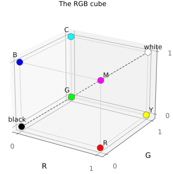
The same matrix idea gives a second, differently-purposed family: the opponent or luma–chroma spaces — YCbCr, YUV, YCoCg — each a fixed $3 \times 3$ map that separates a luma axis from two chroma axes. Splitting brightness from color this way is what lets compression throw away color resolution cheaply (chroma subsampling, since the eye's color acuity is low), and it gives editing tools clean handles. We can even visualize the RGB family geometrically as the RGB cube (Figure 2.5.16), with black at the origin, white at the far corner, and the neutral gray axis running between them.
A caveat to forestall a common confusion: these RGB spaces are related to one another by linear maps (a $3\times3$ matrix), but that is a different sense of "linear" than linear-light. sRGB values carry a gamma; $XYZ$ is linear-light. The two senses of "linear" are independent, and conflating them is a frequent source of color bugs.
2.5.6 Non-linear perceptually-uniform color space⧉
Matrices preserve straight lines but they do not make equal coordinate steps look equally different to the eye. A fixed numerical change in sRGB is a large perceived jump in some colors and an invisible nudge in others. For tasks that need perceptual uniformity — color-difference tolerances, gradients, palette design — we need a deliberately non-linear space. The standard one is CIE L\a\b\ (CIELAB), which applies a cube-root compression of $XYZ$ about a reference white and recombines the result into a lightness axis L\ and two opponent chroma axes a\ (green–red) and b\ (blue–yellow):
Here $(X_n, Y_n, Z_n)$ is the reference white — for D65 and the CIE 1931 2° observer, $(95.047,\,100,\,108.883)$ — and the cube root carries a short linear segment below $\delta^3 \approx 0.0089$ to tame its infinite slope at black. In this space equal distances correspond, roughly, to equal perceived differences, so color difference is just a Euclidean distance, $\Delta E^*_{ab} = \lVert \Delta \mathbf{Lab} \rVert = \sqrt{\Delta L^{*2} + \Delta a^{*2} + \Delta b^{*2}}$ (with the refined ΔE2000 formula correcting the residual non-uniformities). A rough anchor: $\Delta E \approx 1$ is about one just-noticeable difference, and $\Delta E \approx 2.3$ is a common threshold for "acceptable" reproduction. The polar form gives the more intuitive chroma $C^*_{ab} = \sqrt{a^{*2} + b^{*2}}$ (distance from the neutral axis) and hue angle $h_{ab} = \operatorname{atan2}(b^*, a^*)$.
Its close cousin CIE L\u\v\* (CIELUV) keeps the same $L^*$ but scales chromaticity through the CIE 1976 uniform chromaticity coordinates $u', v'$:
with $(u'_n, v'_n)$ the white point's coordinates and $L^* = 116\,(Y/Y_n)^{1/3} - 16$ (again with the linear segment near black, $L^* = (29/3)^3\,Y/Y_n$ when $Y/Y_n \le \delta^3$). CIELUV is favored in lighting and display work because an additive mixture of two lights lies on a straight line in the $u',v'$ plane, so it composes cleanly under addition (Berns, Principles of Color Technology).
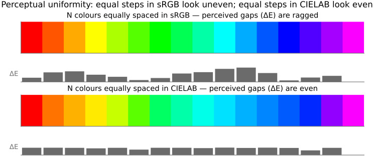
The deeper reason a uniform space must be non-linear is the same reason gamma encoding exists: perception is roughly a power law (Weber–Fechner, Stevens), so any space that turns perceived difference into geometric distance has to warp $XYZ$ accordingly (Figure 2.5.18). CIELAB is not the last word — it has known non-uniformities, especially in saturated blues — and a line of follow-ups refine it while keeping the same intent. The color-appearance-model variant CAM02-UCS (built on CIECAM02) and Björn Ottosson's Oklab improve the perceptual uniformity and the blues; Chong, Gortler & Zickler's perception-based space (Chong et al. 2008) takes a different and, for our purposes, telling angle: it builds a color space from a small set of perceptual axioms and lands on a logarithmic construction that is illumination-invariant — a change of illuminant (which, recall, multiplies the spectrum, L2.6) becomes a simple translation in the space, so the differences image processing cares about are unchanged. That log structure is the same additive-vs-multiplicative theme that runs through tone mapping and exposure, here paying off as robustness to lighting; we use the Chong log space again in gradient-domain compositing.
Concretely, Chong et al. prove that their axioms force the space to be a linear transform of the logarithms of the (linear) cone responses $\boldsymbol{\rho} = (\rho_L, \rho_M, \rho_S)$:
Illumination invariance then fixes $\mathbf{B}$. Under the von Kries model a change of light multiplies each cone channel, $\rho_i \mapsto s_i\,\rho_i$, which in log space is a pure translation $\ln\boldsymbol{\rho} \mapsto \ln\boldsymbol{\rho} + \ln\mathbf{s}$. Choosing $\mathbf{B}$ to project onto the plane orthogonal to the dominant illumination-change direction $\mathbf{d}$ (for a global brightness or color-temperature shift, close to the neutral axis $\mathbf{d} \propto (1,1,1)$),
leaves the chromatic coordinates unchanged by that relighting while a Euclidean distance in $\mathbf{c}$ still approximates a perceptual difference. That is the payoff of the log construction: a change of illuminant becomes a translation, so the color differences image processing depends on are invariant to it.
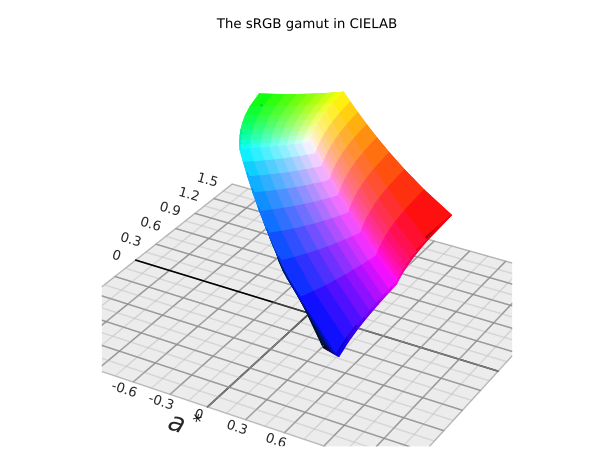
CIELAB warps color to match perceived difference, but perceived color depends on more than the stimulus alone: on the surround, the adapting light, and the brightness. To predict what a color will actually look like, we describe it along its perceptual dimensions, hue, chroma (or colorfulness), and lightness (or brightness), which are just the polar coordinates of the color solid above, radius for chroma and angle for hue around the lightness axis. Color appearance models (CIECAM02 and its successors; see Fairchild, Color Appearance Models) go further, folding in chromatic adaptation and surround effects (the Hunt and Bezold–Brücke phenomena from the perception chapter) to predict appearance across viewing conditions. They are the rigorous engine behind tone mapping and high-end color management, and their uniform variant CAM02-UCS, mentioned above, is one product of the same machinery. Here we need only the vocabulary, hue, chroma, and lightness, and the fact that appearance is not a fixed function of the cone triple. The convenient UI spaces of the next section, HSV and HSL, are cheap approximations of exactly these perceptual axes.
2.5.7 HSV, HSL, and cylindrical color spaces⧉
Not every useful color space aims at perceptual uniformity. The most common ones in software, the hue-saturation-value (HSV) and hue-saturation-lightness (HSL) spaces, are simple cylindrical re-parameterizations of RGB built for convenience rather than measurement. They re-coordinate the RGB cube so that one axis is hue (the angle around the neutral diagonal, running red → yellow → green → cyan → blue → magenta), one is saturation (how far from gray), and one is value or lightness (how bright). Picking a color by turning a hue wheel and then dialing saturation and brightness is far more intuitive than nudging three RGB sliders, which is why almost every color picker is built on HSV or HSL.
The catch is that they are re-parameterizations of gamma-encoded RGB, computed with cheap min/max arithmetic on the R, G, B values, so they inherit all of RGB's non-uniformity and none of CIELAB's perceptual grounding. Equal steps do not look equally different; the "value" and "saturation" axes do not match their perceptual namesakes (a fully saturated yellow and a fully saturated blue share the same HSV value yet differ enormously in real lightness); and the hue angle is not perceptually even. They are excellent for interfaces and quick selections, and misleading the moment you use them for anything quantitative, such as color-difference thresholds, gradients, segmentation, or clustering, where a perceptually grounded space (CIELAB, Oklab) is the right tool. The practical rule mirrors the gamma one: HSV and HSL are fine for choosing colors, but do the math in a space built for it.
2.5.8 Reproducing color⧉
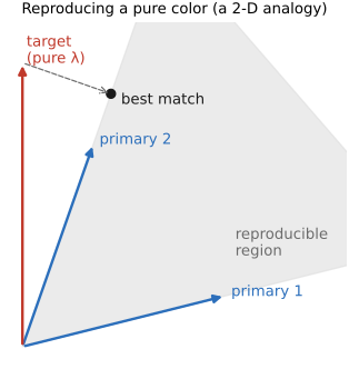
Synthesis, building a color from primaries, is where the constraints of non-orthogonality and non-negativity become concrete. Suppose we want to reproduce a single monochromatic test color, a pure wavelength, using three fixed primaries (Figure 2.5.19). In the linear-algebra picture this is asking for weights $w_i$ such that $\sum_i w_i \mathbf{P}_i$ matches the target. The 2-D analogy makes the trouble plain: with two non-perpendicular basis vectors you can reach any point in the plane if you are allowed negative coefficients — but a primary is a light, and you cannot emit a negative amount of it. So the reachable colors are not the whole plane but only the convex cone of non-negative combinations. Non-orthogonality plus non-negativity turns some perfectly real colors into impossible reproductions: the saturated cyans that needed negative matches in the color-matching experiment simply cannot be made by adding three real primaries.
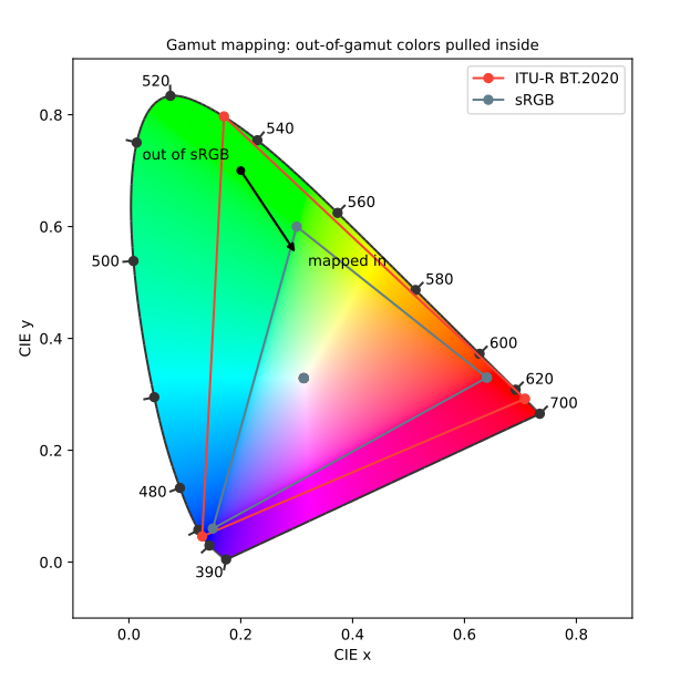
The set of colors a device can make is its gamut: the convex hull of its primaries, the triangle we already saw on the chromaticity diagram (Figure 2.5.14). Colors outside it must be gamut-mapped in (Figure 2.5.20) — clipped to the boundary, or compressed inward to keep relationships, a choice we formalize as rendering intents in the next section.
There are two physically distinct ways to mix color, and the distinction is more subtle than the names suggest. Split the spectrum into three coarse bands and pretend they are pure B, G, R (Figure 2.5.21). Additive mixing — lights — starts from black and adds bands: $R + G + B$ gives white, and the pairs give yellow, cyan, magenta. Subtractive mixing — filters and inks — starts from white and each layer removes a band, with cyan, magenta, yellow stacking toward black. But "subtractive" is a misleading name: stacking filters is really a wavelength-by-wavelength multiplication of the spectrum.
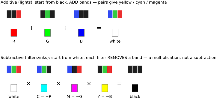
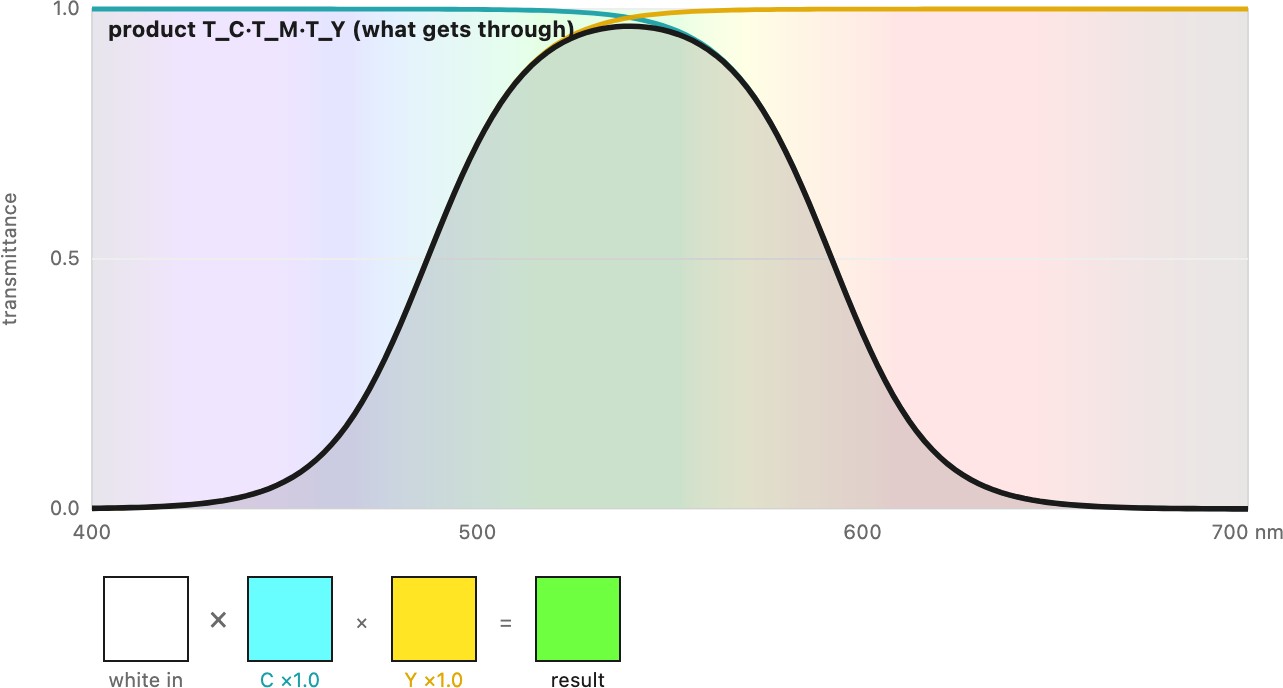
This is easy to see with filter transmittances. A yellow filter blocks blue; a cyan filter blocks red. Stack them and the only band that survives is the overlapping green — so yellow $\times$ cyan = green, which is a product of the two transmittance spectra $T_Y(\lambda)\cdot T_C(\lambda)$, not any kind of sum (Figure 2.5.22). The overlapping-disks picture captures both regimes at a glance: RGB lights overlapping toward white versus cyan-magenta-yellow (CMY) inks overlapping toward black (Figure 2.5.23). And real systems are often hybrid — an LCD projector, for instance, uses a white lamp, panels that subtract (modulate) each channel, and then adds the three channels on the screen.
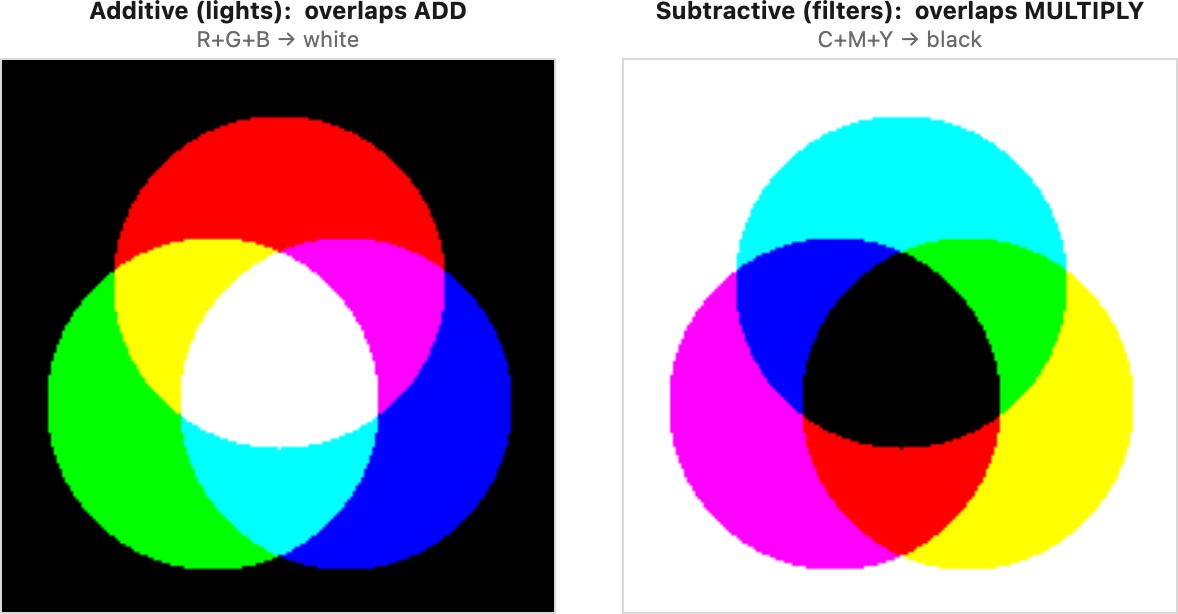
This additive/subtractive split organizes the display and print technologies: CRTs and LCDs and modern OLEDs are additive emitters; projectors come in digital micromirror device (DMD), LCD, and laser flavors; film, printers, and halftoning are subtractive, building tones from overlapping dye or dots. All of them live and die by their gamut and the gamut mapping that squeezes an image into it.
2.5.9 Skin tones⧉
The chapter closes on the color the whole pipeline is quietly tuned around. Skin is a memory color: viewers carry a strong internal expectation of how it should look and notice the slightest error, far more than for grass or sky. Plotted on a vectorscope, skin tones of all people fall along a remarkably tight line — the skin-tone locus, a single hue axis (the I line, between red and orange) — varying mostly in lightness and saturation, not hue (Figure 2.5.24). Cameras and film are deliberately tuned to render that locus pleasingly, which is why "good color science" in a camera is, in large part, good skin.
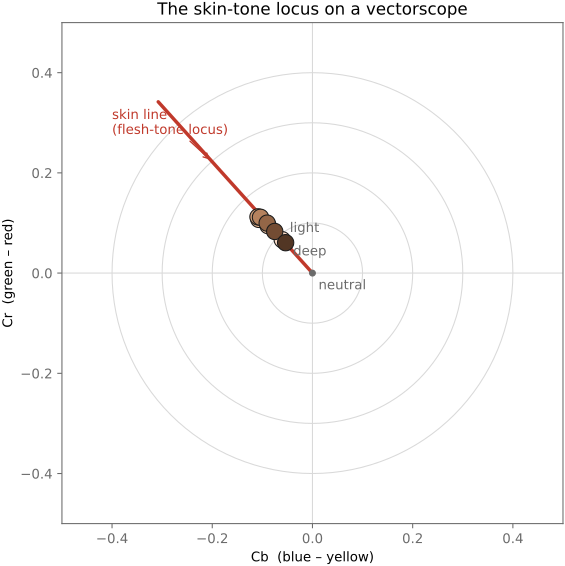
The same tightness shows up in CIELAB, and there it comes with usable numbers (Figure 2.5.25). Skin of every tone sits at nearly the same hue angle, $h_{ab} = \operatorname{atan2}(b^*, a^*) \approx 45\text{–}55°$, a warm red-orange, with positive $a^*$ (redness, roughly $8$ to $18$) and positive $b^*$ (yellowness, roughly $12$ to $26$). What varies from person to person, and with a tan, is mostly the lightness $L^*$ (about $30$ for very dark skin up to $80$ for very light) and the chroma, not the hue. Dermatology compresses this into a single scalar, the individual typology angle,
measured from the neutral point $(L^*{=}50,\, b^*{=}0)$ (Chardon et al. 1991 (ITA°)). ITA° runs from above $55°$ (very light) down through light, intermediate, tan, and brown to below $-30°$ (dark), and is the standard way to place a skin tone on the light-to-dark axis with one number, used from sunscreen testing to dataset-fairness audits.
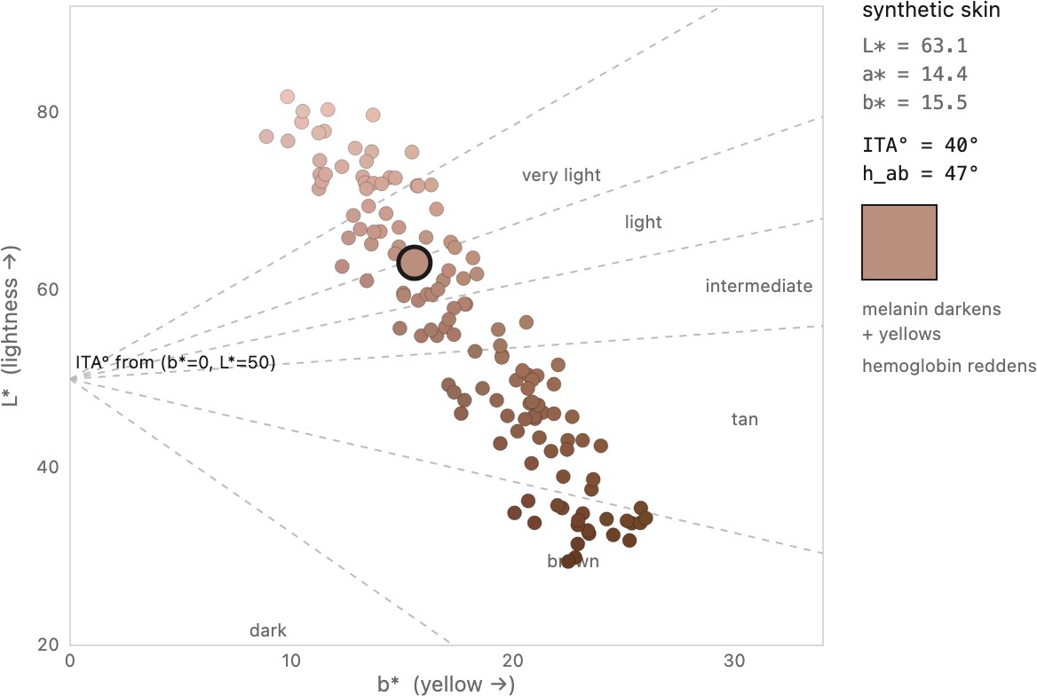
That a skin tone needs essentially two numbers, not three, is not an accident of the color space; it is optics. Skin color is set by just two pigments (chromophores): melanin, in the outer epidermis, a broadband absorber that darkens the skin and pushes it yellow-brown as its concentration rises; and hemoglobin, in the blood of the dermis beneath, which absorbs green light around $540$ to $580$ nm and so contributes the reddish component (and the flush of a blush or of inflammation). Because the reflected light passes through both layers, the observed color is close to a product of a melanin term and a hemoglobin term, which in the log of the sensor responses becomes a sum of two fixed vectors, the same log-of-a-product structure as the Chong space above. Tsumura et al. exploited exactly this: independent component analysis of an ordinary skin photograph recovers separate melanin and hemoglobin density maps, after which skin can be re-lit or retouched by moving along the two chromophore axes independently (Tsumura et al. 2003); the same two-layer model drives physically based skin rendering and the melanin/hemoglobin controls in professional retouching. The locus is one-dimensional in hue precisely because both pigments move a skin tone mainly in lightness and chroma while leaving its hue near that one red-orange line.
Color is only part of the story. Skin does not simply reflect light at its surface, it is translucent: light enters, scatters through the epidermis and dermis, and re-emerges a short distance from where it went in. A per-point surface reflectance (a BRDF) cannot describe that, so a faithful account of skin needs the BSSRDF, the bidirectional surface-scattering reflectance distribution function, which couples an entry point to a separate exit point. That subsurface scattering is what gives skin its soft, lit-from-within glow and its rounded shadow terminator, and rendering a face with a pure surface reflectance instead is exactly why cheap computer-graphics skin looks like plastic (the subsurface-scattering sidebar in Light and physics). Because getting skin right matters so much, a great deal of work has gone into measuring how skin interacts with light, much of it using computational illumination: light stages and light domes that photograph a face under many controlled directions of light and recover its reflectance and subsurface scattering for relighting and realistic rendering (developed in Light domes).
That tuning carries a history the book is obliged to confront. Color film and early video were calibrated against light-skinned reference subjects — the infamous Shirley cards — so that darker skin tones were rendered poorly for decades, a bias baked into chemistry and electronics alike, recounted in the video below. Modern sensors and pipelines render a far wider range of skin faithfully, and should, but the lesson generalizes: a color system tuned for one population fails others unless diversity is designed in from the start. We pick the fairness thread back up in the ethics chapter; here the technical point is that skin is the color by which a whole imaging chain is judged, and rendering it well for everyone is an engineering requirement, not a courtesy.
Recap: big lessons of this chapter
CIE XYZ, the LMS cone responses, and every linear RGB working space (sRGB-linear, Adobe RGB, ProPhoto, a camera's native raw space) are linear transforms of one another — a single $3\times3$ matrix (plus, for a real camera, a fitted approximation). Converting between color spaces is therefore mostly a matrix multiply, and the apparent zoo of color spaces is really one 3-D vector space written in different bases. The non-linear perceptual spaces — CIELAB, the gamma curve — are the deliberate exception, a separate step layered on top (the next sections).
Whether light adds or multiplies should dictate how you encode it. Light from independent sources adds (two lamps, the blur of an out-of-focus lens, the accumulation of photons on a sensor) — these are linear operations, and they are correct only on linear-light values, which is why deconvolution, resizing, and physically-based blur must decode the gamma first. Surface reflectance and perceived contrast, on the other hand, multiply (a gray card under twice the light, a filter cutting a fraction of each wavelength) — and a log encoding makes the multiplicative native, turning products into sums. Gamma is the pragmatic compromise: a power law that behaves better than $\log$ near zero (where $\log$ blows up) while still matching perception. Get this wrong — average gamma values, or sharpen in log — and you get milky blurs, wrong colors, and crushed shadows. The same additive-vs-multiplicative split organizes tone mapping, HDR, and point operations later (→ Big Lessons).