2.6 Pinhole Image Formation and linear perspective⧉
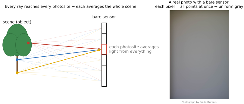
Hold a bare sensor in front of a scene and you get the most blurry image (Figure 2.6.1). And yet light from every object in the scene is landing on that sensor. The trouble is that every point on the sensor receives light from everywhere at once. Each point on the sensor is the average of all the rays in the room, and averaging everything together leaves only a flat, featureless gray.
To make a picture we have to do the opposite of averaging. We must arrange for each point on the sensor to collect light from just one direction, so that each pixel corresponds to one part of the scene. This chapter is about how that selection is done with the crudest possible device, a pinhole, and about the geometry the selection imposes. We will see how a 3D scene flattens into a 2D image by perspective projection (the divide-by-depth that makes distant things small); how that projection becomes a matrix multiply in homogeneous coordinates; what a real camera's intrinsics and extrinsics add, and why cropping a photo is the same as zooming; exactly what perspective preserves (lines and incidence) and what it destroys (angles, lengths, parallelism, hence vanishing points); how a photographer uses focal length to frame and to control the look of the background; and finally how, given depth, we can run the projection backwards and recover 3D points.
2.6.1 Pinhole imaging and the perspective projection⧉
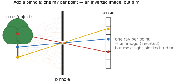
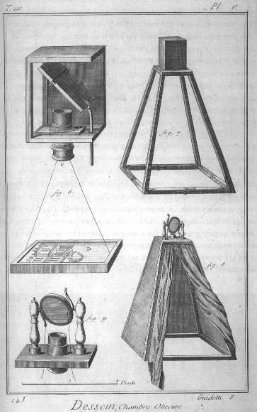
The simplest fix is a wall with a hole in it. Put a barrier between the scene and the sensor and punch a tiny hole, a pinhole, and almost every ray is blocked. For each point on the sensor exactly one ray survives: the single ray from the scene that happens to pass straight through the hole. That one-ray-per-point rule is precisely the selection we needed, and an inverted image appears (Figure 2.6.2). This is the camera obscura (Latin for "dark room"), known to Mozi in ancient China and to Aristotle, used by Renaissance painters as a drawing aid, and still the cleanest way to understand every camera built since (Figure 2.6.5 and Figure 2.6.6). You can make one yourself: a darkened room with a small hole in the window shade projects the street outside, upside down, onto the opposite wall. It is worth doing once, because it makes the geometry below concrete.
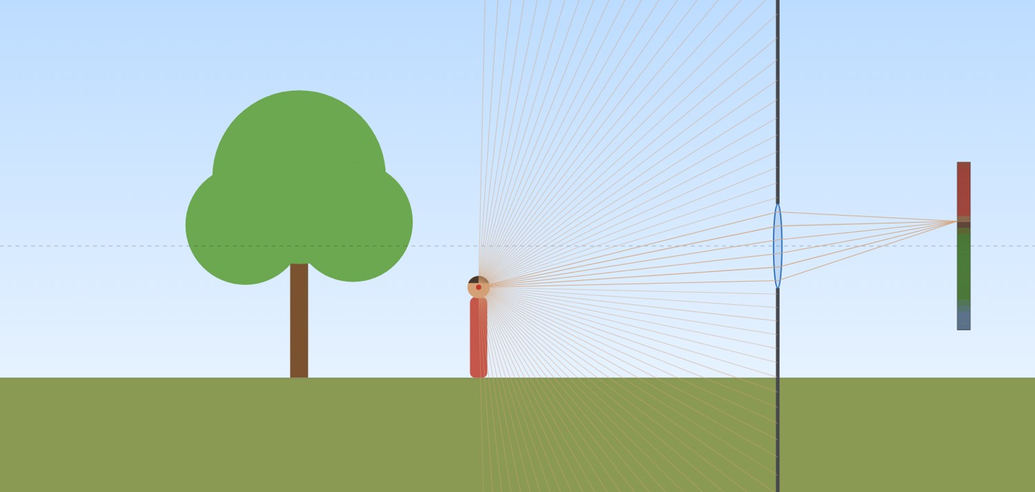
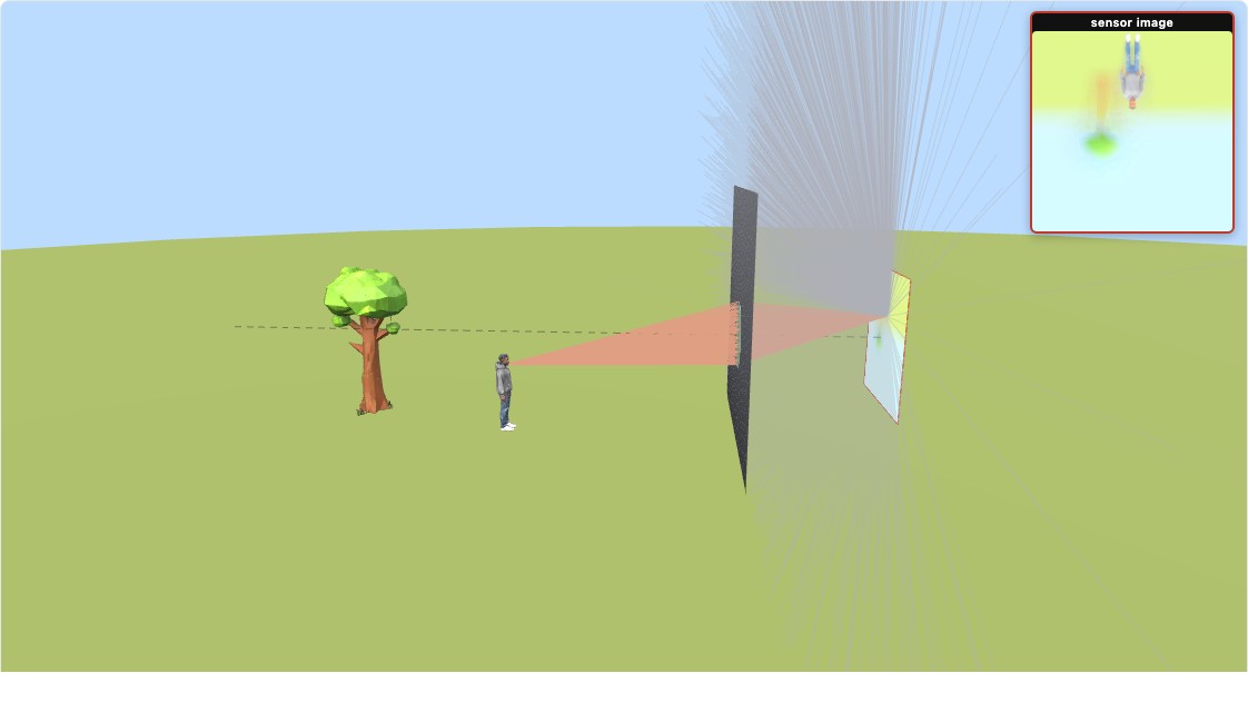
Forming an image is, at bottom, controlling which ray (or rays) of light contribute to each point of the image. A bare sensor fails because every scene point sends light to every pixel. The sum is a flat gray. A pinhole admits one ray per point (sharp, but dim); a lens gathers a whole cone of rays from one scene point and bends them back to one image point (bright, but only for one focal plane); an open hole with no focusing mixes many rays and blurs. Every imaging idea in this book (focus and depth of field, coded apertures, light fields, even a CT scanner) is a different answer to the one question: which rays land here?

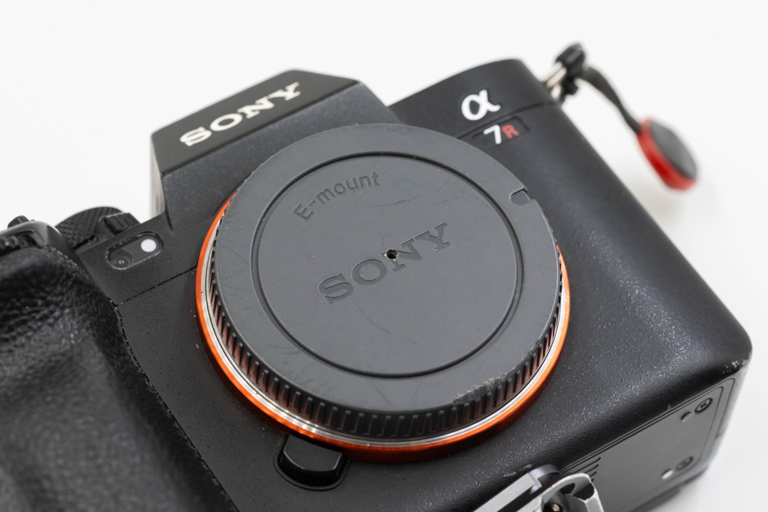
You can still shoot one today: replace a camera's lens with a pinhole and you get a real pinhole photograph (Figure 2.6.7). It reveals the catch the idealized "one ray per point" story hides: a real hole has finite size (and diffraction sets a floor on how small it can usefully be), so each image point actually collects a small disc of rays, not one, so the picture is soft everywhere. But because there is no lens and no focal plane, everything is soft by the same amount: the pinhole has effectively infinite depth of field, the near subject and the far trees equally (un)sharp. A gentle vignetting darkens the corners, where rays strike the sensor at a glancing angle. The result is dim, soft, and has very large depth of field, exactly the trade the lens of the next chapter renegotiates, buying brightness and sharpness at the price of a single plane of focus.

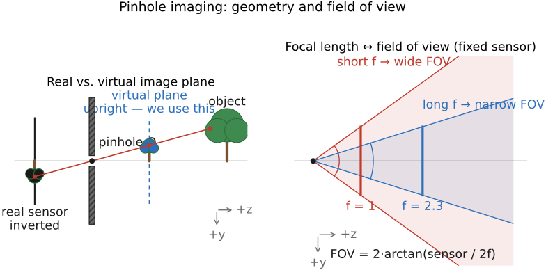
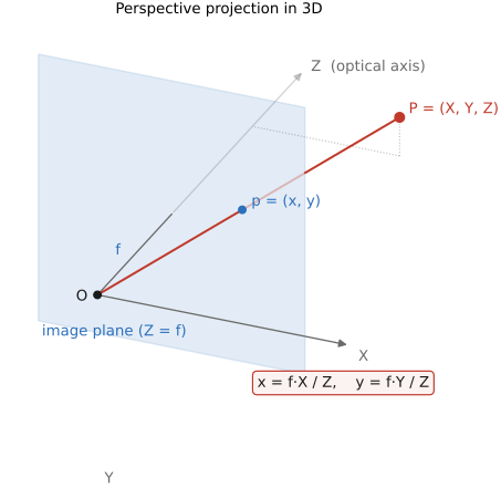
The geometry of a pinhole. To make the picture precise, place the pinhole at the origin and point the camera down the $z$ axis, into the scene, our standing convention (Conventions, Notation & Style#Geometry & coordinate systems: $x$ right, $y$ down, $z$ forward). A scene point sits at world coordinates $(X, Y, Z)$; its one surviving ray runs straight to the pinhole and continues on to strike the sensor. Because the physical sensor sits behind the pinhole, the image it forms is inverted, upside down and flipped left-to-right, exactly as on the wall of the dark room. That inversion is a nuisance to reason about, so throughout the book we use a trick: imagine a virtual image plane the same distance in front of the pinhole. No light actually lands there (it is not physical), but it carries the identical image right-side up, so we never have to mentally flip anything (Figure 2.6.9).
The distance from the pinhole to the image plane controls the field of view for a given sensor size: the bigger it is, the narrower the view. For this purpose it plays exactly the role that the focal length $f$ plays for lenses, so we will use that term throughout, even though, strictly speaking, "focal length" should only apply to lenses. This distance is also what changes when you zoom in or out: a short focal length puts the image plane close to the pinhole, so a wide swath of the scene lands on a sensor of given size (a wide-angle view); a long focal length pushes the plane far away, magnifying a narrow slice (a telephoto view). The exact relation between focal length and the field of view (FOV), for a sensor of a given size, is
which just says: the wider the sensor or the shorter the focal length, the more of the world you take in.
For a pinhole a fixed distance $f$ from the sensor, the field of view is set by the sensor size: $\text{FOV}=2\arctan(\text{sensor}/2f)$. Hold $f$ fixed and slide a larger sensor behind the same pinhole and you take in more of the world; a smaller sensor crops to a narrower view. So "how wide a shot is" is never a property of the pinhole (or, next chapter, the lens) alone: it is the pinhole-to-sensor distance and the sensor size, together. This is the geometric root of the crop factor and of "35 mm-equivalent" focal lengths (next chapter), and the reason the same lens is wide on a big sensor and tele on a small one.
(Pinholes are not merely a teaching device: several animal eyes, such as the nautilus's, are essentially pinhole cameras, trading sharpness for the simplicity of needing no lens; the eye's full evolutionary path (from a bare photoreceptor patch to the lens eye) appears in Animal eyes.)
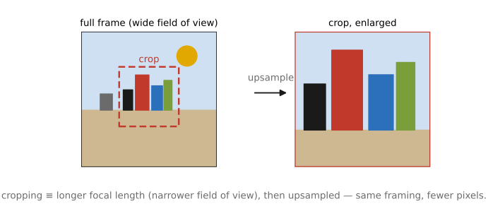
Since zooming is just changing this pinhole-to-sensor distance, it comes to the same thing as cropping: keep the central part of a wider shot, rescale it to fill the frame, and you get exactly the picture a longer focal length would have made (Figure 2.6.10). We will see the formal reason once we split the projection into its pieces, but the equivalence is worth stating now.
From a pure geometric-projection standpoint, cropping an image and zooming in (lengthening the focal length) are one and the same operation. Both leave the perspective projection (the divide-by-$Z$ onto the normalized plane) completely untouched and change only the pixel stage $K$: a crop keeps a smaller patch of the projected image and rescales it to fill the frame, which is exactly what a larger $f_x, f_y$ does. So a 2× crop and a 2× zoom give the identical framing and identical perspective, differing only in resolution: the crop simply has fewer pixels to show for it. This is why "digital zoom" is geometrically free but costs detail, and why the crop factor between sensor sizes acts as a focal-length multiplier.
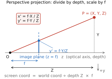
The perspective projection equation. Now read off where a scene point lands. In the side view of Figure 2.6.11, the ray from $(X, Y, Z)$ to the pinhole and the image plane at distance $f$ form two similar triangles. The large triangle has height $Y$ and base $Z$ (the point's height and depth), and the small one has height $y'$, the image coordinate, and base $f$. Similar triangles share their ratio of height to base, so $y'/f = Y/Z$, and the same holds horizontally. The image coordinates of the point are therefore
That is, linear perspective projection of a 3D point consists in a division of its $X$ and $Y$ coordinates by its depth $Z$ and a multiplication by the focal length $f$. This is consistent with higher magnification for a larger focal length and with the foreshortening of points at large depth. That single division by $Z$ is the heart of linear perspective. It is why distant things look smaller (double the depth, halve the image size), why railroad tracks appear to converge, and why a photograph carries a sense of depth that a flat scan of a document does not. Almost everything else in this chapter's geometry is a consequence of dividing by $Z$. The "linear" in linear perspective, by the way, is the painter's term for the rule that straight lines in the world stay straight in the picture, the one nice property the projection keeps, which we make precise two sections from now.
With the camera at the origin looking down $z$, a scene point $(X,Y,Z)$ lands at $(f X/Z,\; f Y/Z)$: the whole of perspective is dividing by depth. That one division produces everything we call perspective: farther things appear smaller (double the depth, halve the size), parallel lines converge to vanishing points, and the picture gains its sense of space. It is also why depth is the hard thing to recover: the division throws $Z$ away, and a single image cannot tell a small near object from a large far one. Every stereo, structure-from-motion, and depth-estimation method in later parts is, in effect, trying to undo this divide.
2.6.2 Homogeneous coordinates⧉
The projection equation is doing something slightly awkward. Multiplying by $f$ is a clean linear operation (a matrix could do it), but the division by $Z$ is not linear, and it makes the projection annoying to compose with the other operations we care about: moving the camera, rotating it, translating the scene. We would like the whole pipeline to be matrix multiplications, because then we can chain and invert them with the linear algebra you already know.
The standard fix is homogeneous coordinates. Write a 2D image point not as $(x, y)$ but as a triple $(x, y, 1)$, and agree that any nonzero scaling of that triple denotes the same point: $(x, y, 1)$, $(2x, 2y, 2)$, and $(wx, wy, w)$ all stand for the same 2D point, recovered by dividing through by the last coordinate. The payoff is that the messy division by $Z$ becomes part of this "divide by the last coordinate" convention, so projection turns into an ordinary matrix multiply followed by the standard homogeneous normalization. As a bonus, translation, which is not a linear operation on ordinary $(x, y)$ coordinates, also becomes a matrix multiply in homogeneous coordinates, which is exactly why all of computer graphics and vision lives in them. We keep the machinery light here; the appendix has the details.
The rule that $(wx, wy, w)$ all mean the same point ("up to scale") is precisely what lets perspective's divide-by-depth hide inside a linear framework: the projection produces a homogeneous triple, and the final divide-through is the division by $Z$. You never lose information by working up to scale: you recover the actual point whenever you need it by normalizing the last coordinate to 1.
Concretely, the perspective projection $x'=fX/Z,\; y'=fY/Z$ becomes a single matrix applied to the homogeneous 3D point $(X,Y,Z,1)$:
The division by $Z$ is now implicit: the result is the homogeneous triple $(fX, fY, Z)$, and the up-to-scale convention recovers the actual image point by dividing through by the last coordinate $w=Z$, giving $(fX/Z,\; fY/Z)$. The awkward nonlinear divide has been swept entirely into the one convention that defines homogeneous coordinates.
A $3\times3$ transformation of ordinary 3D points (a rotation, a scaling, a shear) carries over to homogeneous 4-vectors by padding it out with a $1$ in the extra diagonal slot and zeros elsewhere. A rotation $R$ becomes
a $4\times4$ matrix that rotates the $(X,Y,Z)$ part and leaves the homogeneous weight untouched; any linear map on the coordinates fits this pattern.
Translation is the operation homogeneous coordinates buy us for free. On ordinary coordinates it is not linear (you cannot add a constant with a matrix multiply), yet here it becomes a matrix, with the shift $\mathbf{t}=(t_x,t_y,t_z)$ sitting in the last column:
A rigid camera pose (a rotation and a translation together) is therefore the single $4\times4$ matrix $\left(\begin{smallmatrix} R & \mathbf{t} \\ \mathbf{0}^\top & 1 \end{smallmatrix}\right)$, exactly the extrinsics we meet in the next section.
Surprisingly, this same "carry a value scaled by a weight, then divide it out at the end" trick is exactly how we correctly handle transparency in RGBα images: a pixel's color is stored premultiplied by its alpha, $(\alpha R, \alpha G, \alpha B, \alpha)$, and the true color is recovered by dividing through by $\alpha$, the homogeneous divide all over again. So homogeneous coordinates and premultiplied alpha use the same mathematical pattern, which is why filtering and compositing both insist on it (→ Compositing, segmentation and matting).
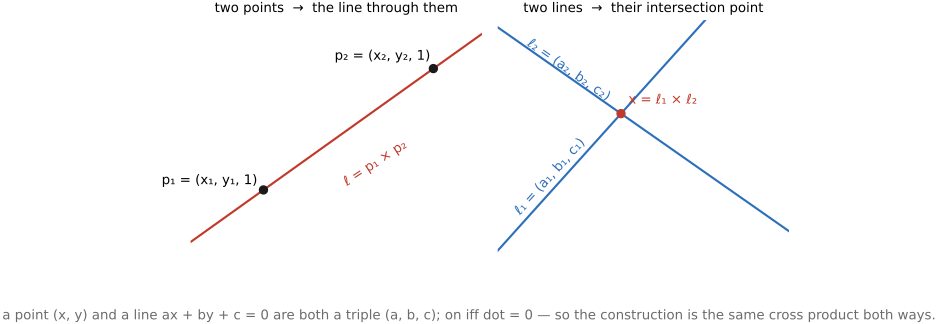
One useful fact follows directly from homogeneous coordinates, and it is worth seeing once because it recurs whenever we fit lines or vanishing points. A line $ax + by + c = 0$ is represented by its triple of coefficients $(a, b, c)$, also up to scale, since scaling the equation does not change the line. So a point is a triple and a line is a triple, and a point lies on a line exactly when their dot product is zero: $(a, b, c)\cdot(x, y, 1) = ax + by + c = 0$. This equation is perfectly symmetric in the point and the line. The consequence is the point↔line duality: two points determine the line through them, and two lines determine their intersection point, by the same cross-product formula (Figure 2.6.13). Anything true of points and lines is true of lines and points. We will quietly lean on this when we compute where parallel lines meet.
2.6.3 Camera in a general configuration⧉
Everything so far assumed the camera sits at the world origin, looking straight down the $+z$ axis. Real cameras are mounted somewhere and pointed somewhere: across the room, tilted up, rolled to one side. The move that handles this is one of the most useful equivalences in all of geometry: moving the camera is the same as moving the world the opposite way. A camera that steps one meter to the right sees exactly what it would see if it stayed put and the whole world slid one meter to the left; a camera that rotates is indistinguishable from a world that counter-rotates around it. The camera's pose and the inverse motion of the world carry the very same information.
That equivalence turns a general camera back into the simple one we already solved. To project from a camera in an arbitrary pose, first apply the inverse of the camera's rigid motion to every world point (this carries the world into the camera's own frame, where the camera once again sits at the origin looking down $z$), and then run the canonical project-and-divide from the previous sections. Two steps: a rigid transform that relocates the world into the camera's coordinate system, followed by the divide-by-depth projection. You can watch the equivalence directly (Figure 2.6.14): drive a camera through a scene and the same view arises two ways at once, once by moving the camera through a fixed world, once by holding the camera at the origin and moving the world by the inverse transform.
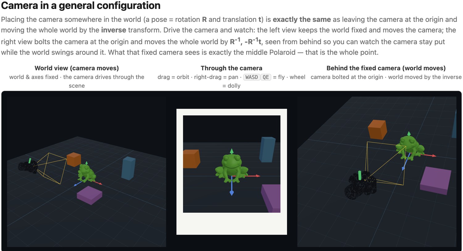
In homogeneous coordinates both steps are linear, so they collapse into a single matrix. Writing a 3D point as a homogeneous 4-vector $(X,Y,Z,1)$, the whole camera (reposition the world, then project) is one $3\times4$ matrix $P$ that produces a homogeneous image triple, from which the actual pixel is read off by the now-familiar divide by the last coordinate. The nonlinearity of perspective has nowhere left to hide: it is only that final division; everything else is a matrix multiply you can compose and invert with the linear algebra you already know.
A camera in any position and orientation projects a 3D point in two moves: a rigid transform that brings the world into the camera's frame (because moving the camera equals moving the world by the inverse), followed by the perspective divide. In homogeneous coordinates the two compose into a single $3\times4$ matrix $P$, applied to the homogeneous point $(X,Y,Z,1)$, and the pixel is recovered by dividing by the last coordinate. So any pinhole view, however the camera is placed, is "one matrix multiply, then one division." That divide is the only nonlinear step in all of projection, the generalization of L2.23's divide-by-depth to an arbitrary viewpoint.
The next section unpacks that single matrix $P$ into its meaningful pieces: the part that depends on where the camera is (its pose, the extrinsics) and the part that depends on the camera and lens themselves (the pixels and focal length, the intrinsics).
2.6.4 Intrinsics, extrinsics, and what cropping really does⧉
The previous section showed that a camera in any configuration is one $3\times4$ matrix $P$ followed by a divide. That matrix bundles everything about the camera together, but it does not yet name the parts. What we want now is a standard way to parameterize all of a camera's degrees of freedom, split cleanly into two kinds. The extrinsics are the camera's pose, where it sits and which way it points, the six degrees of freedom of position and orientation; they change when you move the camera. The intrinsics are properties of the camera and lens themselves, the focal length and where the image is centered; they do not change when you move it. Making the split precise rests on a second distinction we now make explicit: between coordinates measured in world units (meters of scene, and the normalized image coordinates on the $z=1$ plane) and coordinates measured in image units (pixels on the sensor). Untangling those two is the job of the camera matrix, and decomposing $P$ into these stages is also the cleanest way to see why cropping is the same as zooming.
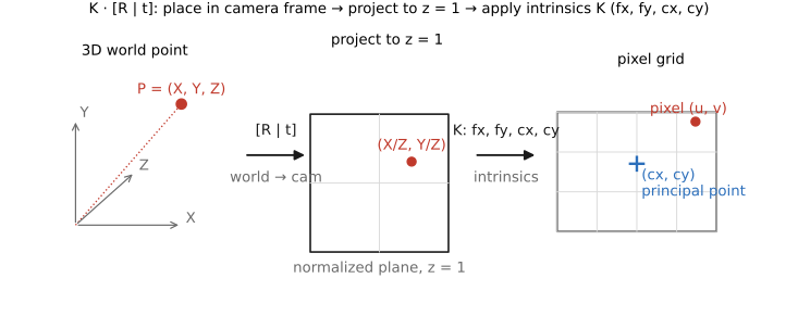
First, reason in normalized image coordinates: project the 3D point straight onto the plane at $z = 1$, with the camera at the origin. This is the bare $x = X/Z$, $y = Y/Z$: pure geometry, with no mention of pixels, sensor size, or focal length. It is the same for every camera.
Second, map those normalized coordinates to actual pixels with a small affine transformation: scale by the focal lengths $f_x, f_y$ (in pixels, possibly different per axis) and shift by the principal point, the pixel location of the image center, which is arbitrary and rarely exactly the middle of the sensor. Stacking these gives the intrinsic matrix $K$. The full projection is then
read right to left: $[R \mid t]$ are the extrinsics, a rotation $R$ and translation $t$ that move the world into the camera's frame (where the camera is, which way it points); the projection at $z=1$ collapses 3D to 2D; and $K$ converts to pixels. Intrinsics are the properties of the camera-and-lens that do not change as you move around: they change only when you zoom or crop; extrinsics are exactly the parameters that change when you move the camera (Figure 2.6.15).
Where the intrinsics live inside the camera, the extrinsics describe its pose in the world: a rigid 6-DOF transform that carries world coordinates into camera coordinates before any projection happens. The rotation $R$ is a $3\times 3$ orthogonal matrix carrying the three degrees of freedom of orientation (which way the camera points and how it is rolled), and the translation $t$ carries the three of position (where it sits). "Moving the camera" is nothing more than changing $R$ and $t$. This is also the machinery that multiple-view geometry rests on: relating two cameras means composing their extrinsics, and the special case of a camera that only rotates (a tripod panning to shoot a panorama, with no translation between shots) collapses $[R \mid t]$ into a pure rotation, so the two views are related by a single $3\times 3$ homography rather than by parallax. That is exactly why a panorama can be stitched from a flat sequence of warps and why it carries no depth information; we take it up in Multiple view geometry and in the chapter on panoramas and homographies.
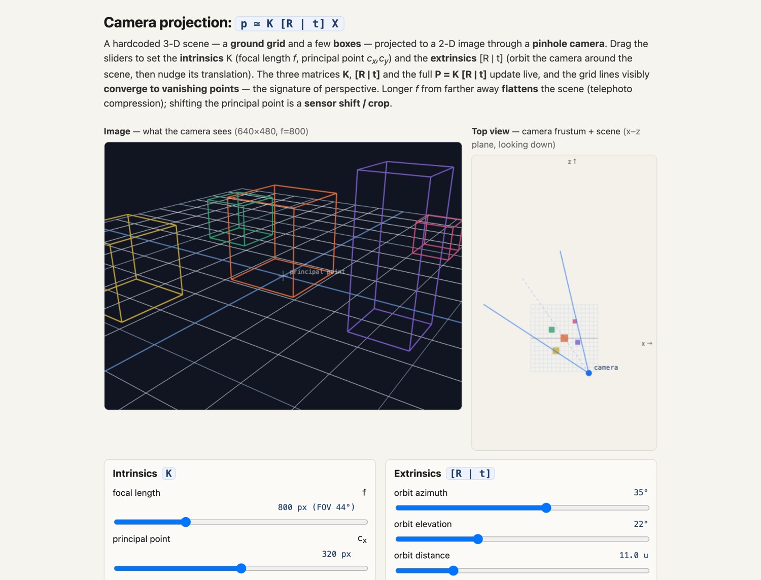
The whole projection equation $p \simeq K[R\mid t]P$ is best felt by driving it yourself: change the intrinsics and watch K change; orbit the camera and watch $[R\mid t]$ change; and at every step the product $P = K[R\mid t]$ updates and the projected scene re-renders, parallels converging to vanishing points (Figure 2.6.16).
This decomposition pays off at once, giving the formal reason behind the crop-equals-zoom equivalence we saw earlier (Figure 2.6.10, Big Lesson L2.22). Because only the second stage, the pixel mapping, knows about the sensor, cropping an image cannot change how the world projects onto the normalized plane; it only keeps a smaller patch of pixels and rescales it to fill the output, which is precisely what increasing $f_x, f_y$ does. A "2× crop" and a "2× zoom" produce the same picture (at lower resolution for the crop). This is also the formal basis for the crop factor that relates sensor sizes, which we return to in the sidebar two sections below.
The extrinsic transform comes in two flavors that are inverses of each other: world-to-camera (where does this world point land in the camera's frame?) and camera-to-world (where in the world is the camera?). A second, sneakier ambiguity rides on top: even within one convention, packages disagree about what $t$ means: some store the camera's actual position, its center $C$ in world coordinates, while the projection $[R \mid t]$ above instead wants its rotated negation, $t = -R\,C$. Datasets and libraries also disagree about whether $y$ points up or down and which axis is forward. Mixing any of these silently flips signs or mirrors a reconstruction (one of the most common bugs in 3D vision), so if you import a pose matrix from someone else's code, pin down which direction it maps and what $t$ means before you trust it.
2.6.5 What perspective preserves, and what it destroys⧉
Perspective projection, the divide-by-$Z$, is a destructive operation, and knowing exactly what it keeps and what it loses is the core intuition behind a great deal of the book.
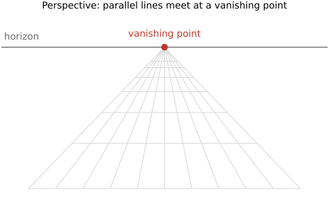
What survives is short: straight lines stay straight (a line in 3D projects to a line in the image), and incidence survives (if a point lay on a line, its image lies on the image of the line). That is essentially all. What is destroyed is more striking: angles and lengths are not preserved. Parallel lines in the world generally do not stay parallel: they converge to a vanishing point. A right angle can project to any angle; a circle can become an ellipse; equal-length fence posts shrink with distance. There is no way to read a true length or a true angle off a single photograph without more information, because the depth that would let you undo the divide-by-$Z$ has been thrown away.
The vanishing point deserves a moment, because it is the most visible signature of perspective. Take a 3D line and march along it toward infinity; its projected image approaches a single fixed point, the vanishing point for that direction. Crucially, every line with the same 3D direction (every member of a family of parallels) marches to the same vanishing point, because in the limit the projection forgets position and keeps only direction. Different directions give different vanishing points; sets of parallel lines lying in a common plane (the ground, say) give vanishing points that all fall on one line, the horizon for that plane (Figure 2.6.17). This is the geometry that painters codified as one-, two-, and three-point perspective, and it is what forced-perspective film tricks exploit, the hobbits-and-Gandalf shots in The Lord of the Rings: place a near object and a far object so they project to plausibly related sizes, and the camera cannot tell they are not the same distance away.
2.6.6 Wide-angle distortion: spheres bulge and faces stretch at the edges⧉
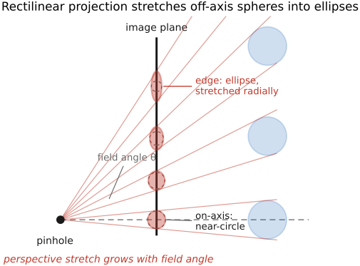
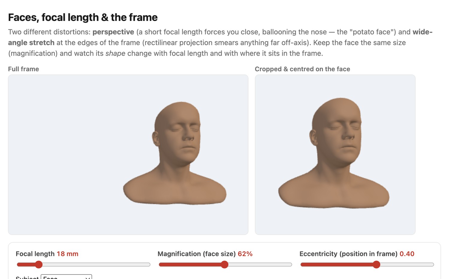
There is a second, subtler distortion hiding in the divide-by-$Z$, and it surprises people because it is not a flaw of any lens. Perspective keeps straight lines straight, but it does not keep solid shapes faithful off-axis. A sphere sitting near the edge of a wide field of view does not image as a circle; it images as an ellipse, stretched radially outward, and the wider the angle the more it bulges. The cause is the flat image plane: a point far off-axis is reached by a ray at a large angle, and projecting that oblique cone onto a flat sensor stretches its footprint. The effect grows with field angle, so it is invisible in a telephoto frame and conspicuous at the edges of a wide-angle one. The everyday giveaway is faces in a wide-angle group photo: the person at the edge looks widened and lurched toward the corner, even though the lens drew every straight line perfectly straight (Figure 2.6.18).
This stretch comes from the projection, not the lens, and that distinction matters. A fisheye "distorts" by bending straight lines; this wide-angle stretch keeps lines straight and is exactly what rectilinear (perspective) projection must do to place an off-axis solid on a flat plane. So no better lens can remove it; only changing the projection can: re-rendering the wide field with a locally stereographic mapping over faces (which keeps shapes round) while leaving straight background lines alone. That content-aware correction is the subject of Perspective distortion and its correction.
The effect on a face is the famous "big nose" of a close wide-angle portrait, and it is best felt by driving it yourself (Figure 2.6.19).
2.6.7 Photography with focal length: framing, magnification, and compression⧉
The projection equation is also a working photographer's toolbox. Focal length sets the field of view, and choosing it is a creative decision: a wide lens (under about 30 mm on full frame) sweeps in a whole landscape and exaggerates near-far size differences; a standard lens (around 50 mm) roughly matches the framing of human attention; a telephoto (over about 100 mm) isolates a distant subject and flattens the scene.
The most useful (and most misunderstood) consequence concerns the difference between focal length and subject distance. Both change how large your subject appears, but they are not interchangeable, because they treat the background differently. Suppose you want a person's face to fill the same fraction of the frame. You can shoot wide and step close, or shoot long and step back. Either way the face is the same size, but stepping close with a wide lens makes the background recede dramatically and the nose loom, while stepping back with a telephoto pulls the background forward until it looks compressed, stacked up right behind the subject (Figure 2.6.20). Portrait photographers prize long lenses for exactly this flattering compression. The effect is not really "the lens compressing space"; it is the change in viewpoint (your distance to the subject) that sets the relative sizes of near and far, while the focal length merely chooses how much of that view to crop. Same subject size, different distance, different background: that is the lever.
You can make a subject fill the same fraction of the frame either by zooming in or by stepping closer, and at that one depth the two give the identical magnification. But magnification falls off with distance, so everything at other depths behaves differently. Changing focal length rescales the whole projected image by a single factor (it is the pixel stage $K$, the "crop = zoom" lesson again), preserving every near-far size ratio; changing your distance rescales near and far by different factors, because each object's magnification depends on its own depth. Step close and the near looms while the far recedes; zoom from afar and the background stacks up "compressed" behind the subject. So relative near-far size (what we call perspective or compression) is set by viewpoint (distance), not by the lens; the focal length only chooses how much of that view to crop. The dolly zoom below is this lesson made vivid.
A related point about sensor size belongs here, even if it feels a touch early. A focal length only means a field of view relative to a sensor size: move the same lens to a smaller sensor and the sensor crops the projected image, narrowing the field of view, the "cropping = longer focal length" fact of Figure 2.6.10, now applied to whole sensors. This is why a focal length on a phone or an APS-C body is usually quoted as a full-frame "equivalent," and it is the perspective that small-sensor cameras give for a stated focal length. The sidebar collects the details.
The field-of-view-depends-on-sensor-size lesson (L2.21) carries straight over to a real lens: for a fixed focal length $f$, the field of view still follows $\text{FOV}=2\arctan(\text{sensor}/2f)$, so the same lens is wide-angle on a big sensor and telephoto on a small one: the smaller sensor simply crops the projected image into a narrower view. A focal length in millimeters therefore says nothing about framing until you also name the sensor, which is why focal lengths are quoted as a 35 mm- (full-frame-) equivalent: the focal length that would frame the same way on a $24\times36$ mm sensor. Concretely, a phone's main camera has an actual focal length of only about 6 mm, but on its tiny (~1/1.3-inch) sensor it frames like a 24–26 mm lens on full frame, so it is sold as "26 mm equivalent." The conversion is just the crop factor, full-frame diagonal ÷ sensor diagonal (≈ 7× for that phone), multiplying the real focal length.
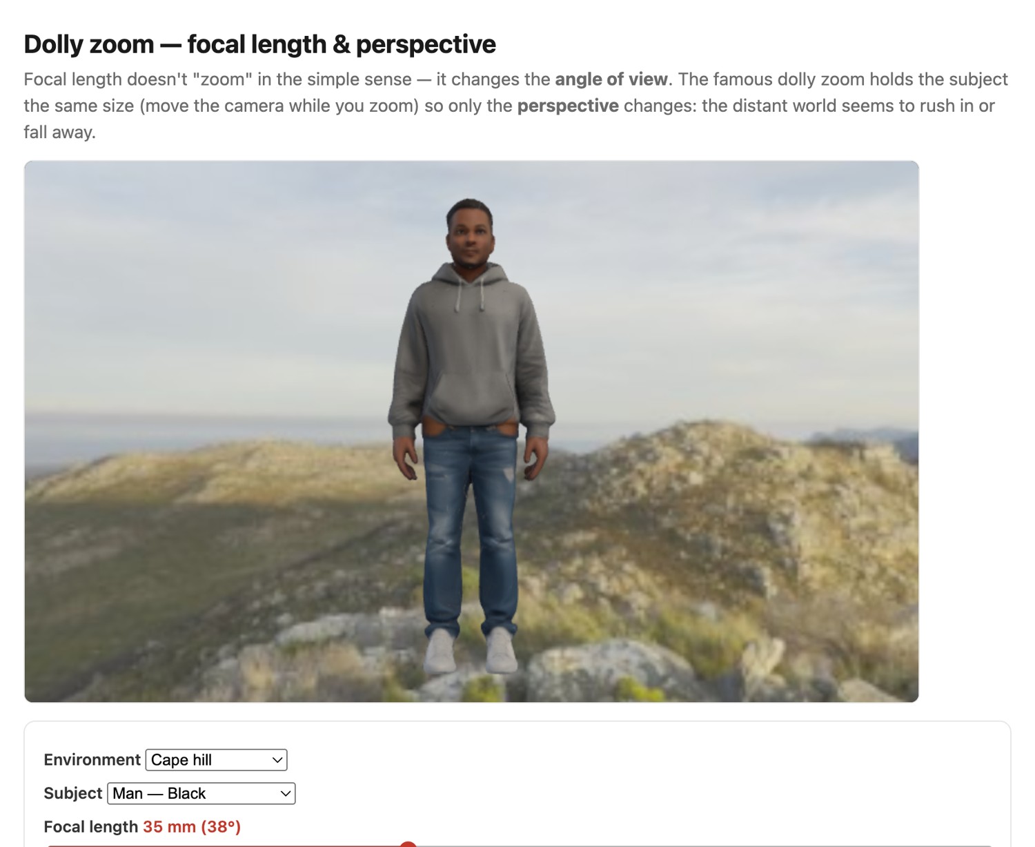
The most vivid demonstration of the lever is the dolly zoom (the "Vertigo" or "trombone" shot): zoom in while dollying the camera back (or out while moving in) so the subject stays exactly the same size while the background visibly rushes in or pulls away behind it. Because only the viewpoint distance is changing, the subject is pinned while the world behind it expands or contracts, the focal-length-vs-distance trade-off, animated (Figure 2.6.21).
Photographers call a $24 \times 36$ mm image frame "35 mm," which sounds like a contradiction. The "35 mm" is the width of the film stock, including the sprocket-hole margins, not the image. Oskar Barnack, designing the first Leica, ran 35 mm cine film sideways through a still camera, giving a 36 mm × 24 mm frame. Today that size is called full frame, and smaller sensors are quoted by their crop factor relative to it: APS-C is about 1.5×, its name coming from the old Advanced Photo System (APS) film format, Micro Four Thirds about 2×, and a phone sensor much smaller still. The crop factor is just the "cropping = longer focal length" fact of Figure 2.6.10 applied to sensor sizes: a 50 mm lens on an APS-C body frames like a 75 mm lens on full frame, because the smaller sensor crops the projected image.
2.6.8 Depth, ray length, and unprojection⧉
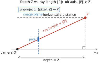
One subtlety trips up everyone who works with depth data, so we flag it now. The depth of a scene point is its $Z$ coordinate, its distance along the optical axis, the thing we divided by. It is not the length of the ray from the camera to the point. A point off to the side of the frame has a longer ray than a point dead ahead at the same $Z$, because the ray runs diagonally. Depth sensors, and depth maps generally, report $Z$, not ray length; keeping the two distinct saves a great deal of grief.
With $Z$ in hand, you can invert the projection. The forward map $x' = fX/Z$ loses depth: many 3D points share an image point, namely all the points along one ray. But give the depth back, and a pixel plus a depth determines a unique 3D point. Solving $x' = fX/Z$ for $X$ (and likewise for $Y$) recovers $X = x'Z/f$, $Y = y'Z/f$: this is unprojection, and it is what a depth camera such as an Intel RealSense does live, turning each pixel-plus-depth into a 3D point cloud (Figure 2.6.22). Such sensors recover $Z$ in several ways, stereo (a later chapter), structured light, or time-of-flight, but once they have it, unprojection is the same simple arithmetic for all of them. This forward-and-back pair (project to lose depth, unproject to restore it given $Z$) is the bridge from this chapter's one-camera geometry to the multiple-view geometry that measures the missing depth.
With the geometry of a single pinhole in hand (how the world flattens, what survives, and how to run it backwards given depth), we are ready for the device that replaces the pinhole. The next chapter swaps the light-starved hole for a lens, which gathers a wide cone of light and focuses it, buying brightness at the cost of a single plane of focus and a finite depth of field. The projection geometry of this chapter carries over unchanged: a lens, to first order, has exactly the pinhole's perspective.
Recap: big lessons of this chapter
Forming an image is, at bottom, controlling which ray (or rays) of light contribute to each point of the image. A bare sensor fails because every scene point sends light to every pixel. The sum is a flat gray. A pinhole admits one ray per point (sharp, but dim); a lens gathers a whole cone of rays from one scene point and bends them back to one image point (bright, but only for one focal plane); an open hole with no focusing mixes many rays and blurs. Every imaging idea in this book (focus and depth of field, coded apertures, light fields, even a CT scanner) is a different answer to the one question: which rays land here?
For a pinhole a fixed distance $f$ from the sensor, the field of view is set by the sensor size: $\text{FOV}=2\arctan(\text{sensor}/2f)$. Hold $f$ fixed and slide a larger sensor behind the same pinhole and you take in more of the world; a smaller sensor crops to a narrower view. So "how wide a shot is" is never a property of the pinhole (or, next chapter, the lens) alone: it is the pinhole-to-sensor distance and the sensor size, together. This is the geometric root of the crop factor and of "35 mm-equivalent" focal lengths (next chapter), and the reason the same lens is wide on a big sensor and tele on a small one.
From a pure geometric-projection standpoint, cropping an image and zooming in (lengthening the focal length) are one and the same operation. Both leave the perspective projection (the divide-by-$Z$ onto the normalized plane) completely untouched and change only the pixel stage $K$: a crop keeps a smaller patch of the projected image and rescales it to fill the frame, which is exactly what a larger $f_x, f_y$ does. So a 2× crop and a 2× zoom give the identical framing and identical perspective, differing only in resolution: the crop simply has fewer pixels to show for it. This is why "digital zoom" is geometrically free but costs detail, and why the crop factor between sensor sizes acts as a focal-length multiplier.
With the camera at the origin looking down $z$, a scene point $(X,Y,Z)$ lands at $(f X/Z,\; f Y/Z)$: the whole of perspective is dividing by depth. That one division produces everything we call perspective: farther things appear smaller (double the depth, halve the size), parallel lines converge to vanishing points, and the picture gains its sense of space. It is also why depth is the hard thing to recover: the division throws $Z$ away, and a single image cannot tell a small near object from a large far one. Every stereo, structure-from-motion, and depth-estimation method in later parts is, in effect, trying to undo this divide.
A camera in any position and orientation projects a 3D point in two moves: a rigid transform that brings the world into the camera's frame (because moving the camera equals moving the world by the inverse), followed by the perspective divide. In homogeneous coordinates the two compose into a single $3\times4$ matrix $P$, applied to the homogeneous point $(X,Y,Z,1)$, and the pixel is recovered by dividing by the last coordinate. So any pinhole view, however the camera is placed, is "one matrix multiply, then one division." That divide is the only nonlinear step in all of projection, the generalization of L2.23's divide-by-depth to an arbitrary viewpoint.
You can make a subject fill the same fraction of the frame either by zooming in or by stepping closer, and at that one depth the two give the identical magnification. But magnification falls off with distance, so everything at other depths behaves differently. Changing focal length rescales the whole projected image by a single factor (it is the pixel stage $K$, the "crop = zoom" lesson again), preserving every near-far size ratio; changing your distance rescales near and far by different factors, because each object's magnification depends on its own depth. Step close and the near looms while the far recedes; zoom from afar and the background stacks up "compressed" behind the subject. So relative near-far size (what we call perspective or compression) is set by viewpoint (distance), not by the lens; the focal length only chooses how much of that view to crop. The dolly zoom below is this lesson made vivid.
The field-of-view-depends-on-sensor-size lesson (L2.21) carries straight over to a real lens: for a fixed focal length $f$, the field of view still follows $\text{FOV}=2\arctan(\text{sensor}/2f)$, so the same lens is wide-angle on a big sensor and telephoto on a small one: the smaller sensor simply crops the projected image into a narrower view. A focal length in millimeters therefore says nothing about framing until you also name the sensor, which is why focal lengths are quoted as a 35 mm- (full-frame-) equivalent: the focal length that would frame the same way on a $24\times36$ mm sensor. Concretely, a phone's main camera has an actual focal length of only about 6 mm, but on its tiny (~1/1.3-inch) sensor it frames like a 24–26 mm lens on full frame, so it is sold as "26 mm equivalent." The conversion is just the crop factor, full-frame diagonal ÷ sensor diagonal (≈ 7× for that phone), multiplying the real focal length.