4.11 Sampling, downsampling, and aliasing⧉
A digital image is a sampling of a continuous scene — we record the value on a regular grid and throw away everything in between. Most of the time that is harmless. But when the scene carries detail finer than the grid can resolve, something counter-intuitive happens, and it is one of the most surprising facts in imaging. The previous chapter built the Fourier machinery; sampling is the thing that machinery explains most cleanly, because a sampling grid is just a comb of evenly shifted spikes. (We treat the reconstruction / upsampling direction — putting values between samples — in the next chapter, Resampling; here the concern is what goes wrong when we throw samples away.)
4.11.1 Aliasing: a high frequency in disguise⧉
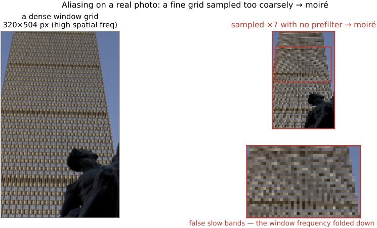
Picture photographing a building's facade — rows of fine windows, or a striped shirt — and shrinking the result. Where the stripes are finer than the output pixels, they do not melt into a uniform gray; they reorganize into bold, wrong, low-frequency bands and swirls that are not in the scene at all: moiré. Intuitively, when a pixel must summarize detail it cannot represent, it ought to return the local average — a neutral gray. Instead, the leftover high frequency gets misread as a low one.
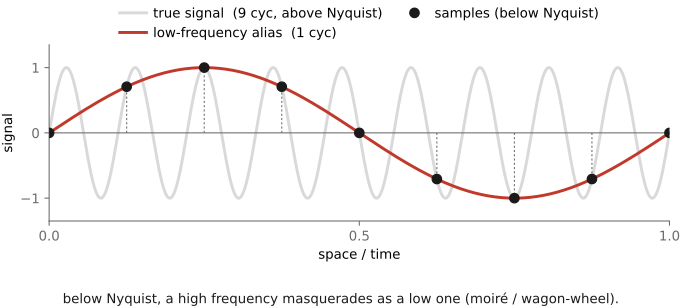
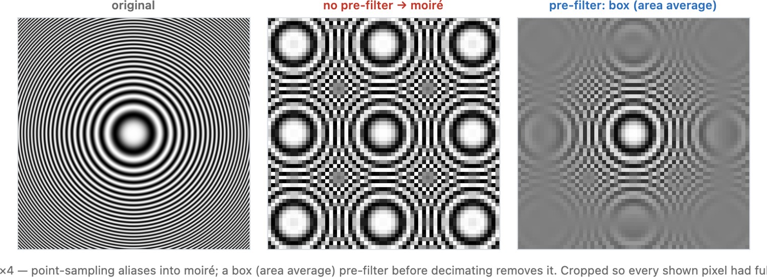
The clean case is a single sine wave (Figure 4.11.1). Sample a high-frequency sine too coarsely — fewer than two samples per cycle — and the samples you collect fall into a pattern indistinguishable from a lower-frequency sine. The original travels in disguise as a different frequency; that impostor frequency is its alias. The damage is not blur (lost detail you could shrug off); it is corruption — energy that lands at the wrong frequency and masquerades as real structure. The same masquerade plays out in 2-D on a real photograph (Figure 4.11.2): a facade's regular window grid is a high spatial frequency, and sampling it too coarsely without a pre-filter folds that grid down into bold, slow moiré bands that are not in the building.
4.11.2 Nyquist and the sampling theorem⧉
The rule that prevents it is the Nyquist–Shannon sampling theorem: to represent a signal faithfully you must sample at more than twice its highest frequency. Equivalently, with a fixed sampling grid there is a top frequency — the Nyquist frequency, half the sampling rate — that the grid can represent; anything above it cannot be stored and, if present, folds (aliases) down onto a lower frequency and contaminates it. There is no recovering from aliasing after the fact: once a high frequency has folded onto a low one, the two are added together and can never be told apart.
To represent a signal from its samples you must sample at more than twice its highest frequency (the Nyquist rate). Sample any slower and the frequencies above the Nyquist limit (half the sampling rate) cannot be stored — they fold down and alias onto lower frequencies, masquerading as structure that is not there (the moiré on a fine facade, the backward wagon-wheel). This is the spatial root lesson of all sampling, and it is not confined to space: the very same theorem governs the time axis, where under-sampling a fast motion gives temporal aliasing — the wagon-wheel and rotor-freeze effects of film and video. The only cure is to band-limit before you sample: low-pass (blur / area-average) away everything above Nyquist first, then sample (the anti-aliasing prefilter, L16). The frequency-domain account of why — sampling replicates the spectrum and the copies overlap — is L4.13; the ideal band-limiting filter, the unreachable sinc, is L4.14.
The theorem cuts both ways, which is why it is so central. It tells you when sampling is safe — the signal is already band-limited below Nyquist, so nothing folds — and exactly what to do when it is not: kill the offending frequencies before they fold. And because it is a statement about any sampled signal, it reappears far beyond image shrinking: in audio (the 44.1 kHz CD rate is a little over twice the ~20 kHz of human hearing), in video frame rates, and — on the time rather than the space axis — as the temporal aliasing we just named.
4.11.3 In two dimensions, aliasing has a direction⧉
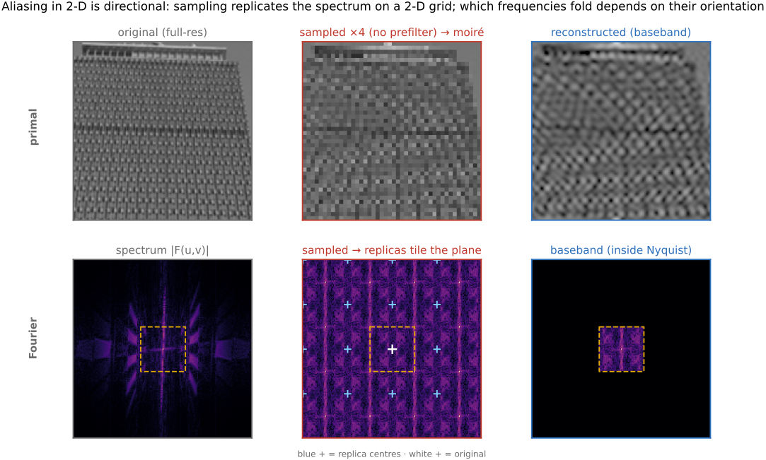
Everything so far has been the 1-D story — a fast sine masquerading as a slow one — and in 1-D there is only one thing an alias can do: land at a lower frequency along the single axis. In two dimensions it is messier, because a spatial frequency carries not just a rate but a direction, and aliasing folds both. A 2-D high frequency does not simply drop to a lower 2-D frequency; it folds to a frequency with a possibly different orientation. So a perfectly regular pattern can alias into moiré that runs in an unexpected direction — diagonal bands from a vertical grille, swirling rosettes from concentric rings — bearing no obvious relation to the orientation of the detail that produced it. The aliases of a 2-D signal do not share a single direction the way the 1-D alias shares the lone axis, which is exactly why 2-D moiré looks so strange: each folded frequency arrives pointing its own way.
The canonical directional case is the humblest one: the stair-step or "jaggies" on a near-horizontal or near-vertical edge. A slightly slanted edge is, locally, a very low-frequency ramp crossed by a high-frequency component along the edge; sample it on the pixel grid without prefiltering and that high frequency folds, breaking the smooth slant into a staircase of horizontal and vertical pixel runs. The jaggy is aliasing wearing its plainest costume — and the reason anti-aliasing in rendering and rasterization is, at heart, the same band-limit-then-sample prefilter we are building here, applied to synthetic edges instead of a photographed facade.
4.11.4 Sampling in the frequency domain: spectral replicas⧉
In the frequency domain the mechanism is vivid. Sampling on a grid is multiplying the signal by a comb of spikes, and multiplying by a comb in space replicates the spectrum — it pastes shifted copies of the signal's spectrum at every multiple of the sampling rate. If the original spectrum is narrow enough (band-limited below Nyquist), the copies sit side by side without touching and the original can be isolated. If it is too wide, the copies overlap, the tails fold back over the genuine low frequencies, and that overlap is aliasing. Seen this way the fix is obvious: band-limit the signal before you sample it. Run a low-pass filter — a blur — first, to delete the frequencies above Nyquist that would otherwise fold, then sample. This pre-filter (anti-aliasing) trades a little sharpness for the removal of false structure, and it is why a well-written image-shrinking routine blurs before it downsamples. The space-versus-frequency tradeoff returns: a perfectly sharp cutoff in frequency is a sinc spread out forever in space, so practical pre-filters compromise.
Sampling on a grid is multiplication by a comb (a train of deltas), and a comb's Fourier transform is another comb — so sampling replicates the signal's spectrum at every multiple of the sampling rate. If the spectrum is band-limited below Nyquist the copies sit side by side and the original is recoverable; if it is not, the copies overlap, and the folded-over tails land on top of the genuine low frequencies as aliasing — energy appearing at completely wrong frequencies (moiré, the backward wagon-wheel). The cure is to band-limit before sampling: low-pass away everything above Nyquist first, then sample.
4.11.5 Seeing it: sampling and pre-filtering, hands on⧉
The demos below show this directly. The first demo is the one-dimensional story — a single signal, your hand on the sampling rate — and the second is the two-dimensional one, the same physics on a real photograph where aliasing shows up as moiré.
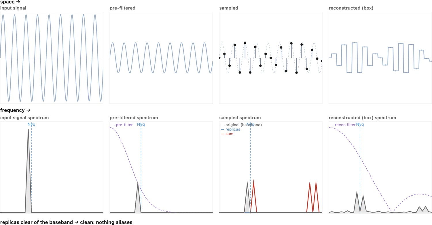
The full sampling pipeline generalizes to two dimensions just as cleanly, and the spectral picture is the most revealing part: in 2-D, sampling replicates the spectrum on a whole lattice of copies, and aliasing is a copy drifting in to overlap the baseband.
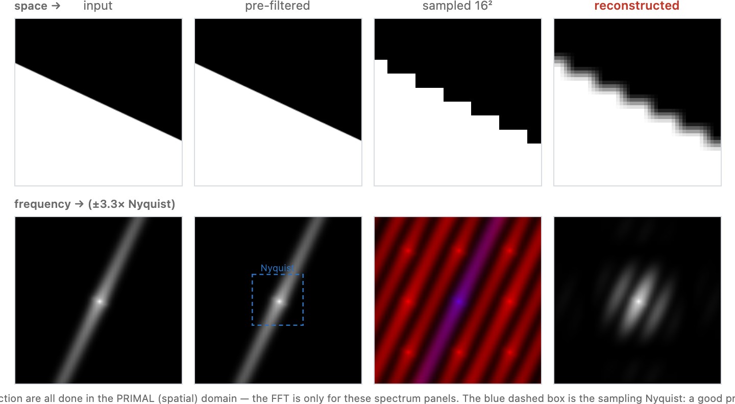
You do not strictly need Fourier to feel why sampling fails. A pixel records the signal at a single point, not the average over its little footprint, so two scenes that happen to agree at every sample point produce identical images even if they differ wildly in between — a fast wiggle and a slow one can thread the same dots. The correct "what should a pixel be?" answer is the average over the pixel's area (the integral of the scene under the pixel's footprint), and computing that average is the pre-filtering blur described above, dressed in primal-domain clothes. Fourier merely turns this geometric coincidence into a precise statement about which frequencies survive.
Everything so far has treated aliasing as a nuisance to be suppressed. But the same effect can be engineered to carry information. Print a fine micro-pattern, photograph it with a camera, and the camera's own pixel grid samples that pattern too coarsely — producing a moiré that is no longer in the print at all but emerges from the beat between the print's spatial frequency and the sensor's sampling grid. Because that beat pattern is exquisitely sensitive to the exact sampling geometry, it shifts dramatically with the slightest change in viewpoint — so the moiré effectively encodes the relative camera pose or motion, reading out information that the bare pixels never recorded. MIT's KinéCam dynamic prints exploit exactly this: a static printed micro-pattern that animates and reports camera motion entirely through engineered moiré (hcie.csail.mit.edu/research/kinecam). It is the same physics as the wagon wheel and the striped shirt, turned from a bug into a channel — and it rhymes with the structured / coded patterns that recur elsewhere in the book.
4.11.6 The ideal reconstruction filter: sinc, and why it is unreachable⧉
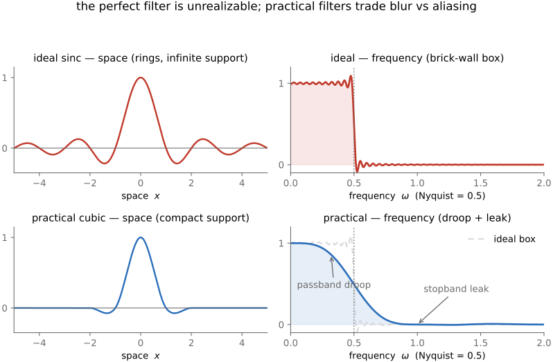
The deepest reconstruction filter, the one Nyquist's theorem secretly invokes, is the sinc: in the frequency domain it is a perfect box — keep everything below Nyquist, kill everything above, with a vertical wall in between. The sinc reconstructs a band-limited signal exactly. But that vertical frequency wall costs a kernel that ripples on forever in space (the space–frequency tradeoff again), and infinitely wide kernels are neither practical nor well-behaved — they ring. So real systems use approximations to the sinc with finite support (Figure 4.11.7), each striking its own bargain between losing a little mid-frequency contrast and letting a little high-frequency aliasing through. We will meet the practical menagerie — bilinear, bicubic, Lanczos — in the resampling chapter; here the point is only that the ideal exists, that it is unreachable, and that every real filter is a compromise away from it.
Both jobs sampling demands — the anti-alias pre-filter (a perfect low-pass before sampling) and the reconstruction filter (a perfect low-pass to interpolate between samples) — have the same mathematically ideal answer: the sinc, a perfect brick-wall box in frequency. But a vertical wall in frequency is an infinitely wide, forever-ringing kernel in space (the space–frequency tradeoff again), so the ideal is physically unreachable: you cannot store or convolve an infinite kernel, and truncating it makes it ring. Every real pre-filter and every real resampling kernel — box, bilinear, bicubic, Lanczos — is therefore a compromise away from the sinc, trading a little lost mid-frequency contrast against a little leaked aliasing. There is no free lunch and no perfect filter; choosing one is choosing which error to tolerate.
Recap: big lessons of this chapter
To represent a signal from its samples you must sample at more than twice its highest frequency (the Nyquist rate). Sample any slower and the frequencies above the Nyquist limit (half the sampling rate) cannot be stored — they fold down and alias onto lower frequencies, masquerading as structure that is not there (the moiré on a fine facade, the backward wagon-wheel). This is the spatial root lesson of all sampling, and it is not confined to space: the very same theorem governs the time axis, where under-sampling a fast motion gives temporal aliasing — the wagon-wheel and rotor-freeze effects of film and video. The only cure is to band-limit before you sample: low-pass (blur / area-average) away everything above Nyquist first, then sample (the anti-aliasing prefilter, L16). The frequency-domain account of why — sampling replicates the spectrum and the copies overlap — is L4.13; the ideal band-limiting filter, the unreachable sinc, is L4.14.
Sampling on a grid is multiplication by a comb (a train of deltas), and a comb's Fourier transform is another comb — so sampling replicates the signal's spectrum at every multiple of the sampling rate. If the spectrum is band-limited below Nyquist the copies sit side by side and the original is recoverable; if it is not, the copies overlap, and the folded-over tails land on top of the genuine low frequencies as aliasing — energy appearing at completely wrong frequencies (moiré, the backward wagon-wheel). The cure is to band-limit before sampling: low-pass away everything above Nyquist first, then sample.
Both jobs sampling demands — the anti-alias pre-filter (a perfect low-pass before sampling) and the reconstruction filter (a perfect low-pass to interpolate between samples) — have the same mathematically ideal answer: the sinc, a perfect brick-wall box in frequency. But a vertical wall in frequency is an infinitely wide, forever-ringing kernel in space (the space–frequency tradeoff again), so the ideal is physically unreachable: you cannot store or convolve an infinite kernel, and truncating it makes it ring. Every real pre-filter and every real resampling kernel — box, bilinear, bicubic, Lanczos — is therefore a compromise away from the sinc, trading a little lost mid-frequency contrast against a little leaked aliasing. There is no free lunch and no perfect filter; choosing one is choosing which error to tolerate.