2.3 Human Vision🔗⧉

Where Perceptual color and trichromatic vision asked what color is this, this chapter asks what the visual system does with light and color once it has them: it adapts to the overall level, discounts the illuminant to recover the reflectance of surfaces (lightness and color constancy), works in ratios rather than absolutes (contrast), and resolves detail unevenly across spatial and temporal frequency (the contrast sensitivity functions). These are the properties that let compression, tone mapping, and quality metrics optimize for the eye rather than for pixels.

2.3.1 Light adaptation🔗⧉

The eye faces a dynamic range that no single setting could span — starlight to direct sun is a factor of billions. It copes not by capturing it all at once but by adapting over time, continually recentering its response around the current average brightness. Walk into a dark cinema and you are blind for a minute, then the seats swim into view; step back out and the lobby is blinding before it settles. The neural response to intensity $I$ is well described by a saturating (Naka–Rushton) curve Naka & Rushton 1966,

an S-shaped function whose half-saturation point $I_0$ slides to track the prevailing light — so the limited response range is always spent where it is useful.

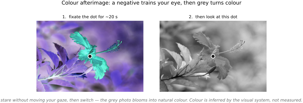
Three mechanisms cooperate across different timescales: neural gain control (fast), photochemical bleaching and regeneration of the photopigment (slower — the minutes of dark adaptation), and the pupil (a quick but small contribution, a couple of stops at most). The consequences are everywhere: afterimages again (a local adaptation that leaves a stamp when the gaze moves), and striking illusions of motion such as the Spanish-Castle illusion, where staring at a color-reversed image and then a blank field produces a fleeting full-color positive — adaptation of the opponent channels writ large (Figure 2.3.1). Adaptation is why the eye's "dynamic range" is so often overstated: it is huge over time, far smaller in any single instant — exactly the gap that high-dynamic-range (HDR) capture and tone mapping (later chapters) must bridge.

Where the eye operates also changes which receptors do the work, and we name three regimes by the prevailing luminance (in candela per square meter, $\text{cd/m}^2$ — the photometric "nit" from Light and physics, light measured along a ray). They are (Figure 2.3.2):

• Photopic (daylight): the cones are in charge, giving full color and sharp foveal vision. Roughly above $3\,\text{cd/m}^2$ — office light sits near $10^{2}$, an overcast sky around $10^{3}$–$10^{4}$, a sunlit scene around $10^{4}$–$10^{5}\,\text{cd/m}^2$.
• Mesopic (dusk or a dim interior): rods and cones work together, roughly $10^{-3}$ to $3\,\text{cd/m}^2$. Colors desaturate and the Purkinje shift sets in — as rods take over, blues look relatively brighter and reds relatively darker (the flowers that glowed red at noon go murky at dusk while the blue foliage stays luminous).
• Scotopic (night): rods only — no color, poor acuity, and notably off-fovea, since the all-cone fovea is effectively blind in the dark (which is why a faint star vanishes when you look straight at it). Below about $10^{-3}\,\text{cd/m}^2$ — a moonlit landscape near $10^{-2}$, starlight around $10^{-3}$–$10^{-4}$, and the absolute threshold of vision down near $10^{-6}\,\text{cd/m}^2$ (a handful of photons).

The overall range is large: across these regimes the eye works over roughly $10^{-6}$ to $10^{8}\,\text{cd/m}^2$ — about 14 log units of luminance — yet it spans only a few log units at any one instant. That gap between the total range and the instantaneous range is precisely why adaptation exists in the eye, and precisely why cameras need high-dynamic-range (HDR) capture and tone mapping (later chapters) to pack a scene's range into a display's.

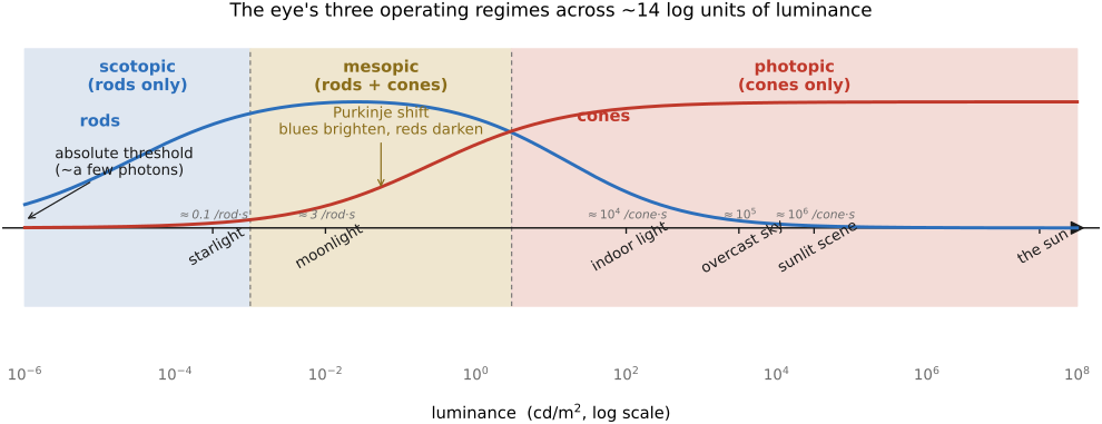
It is worth turning these luminances into the currency the receptors actually deal in: photons. A luminance in cd/m² becomes a photon rate once you account for the pupil (the iris), which narrows from about $7\,$mm in the dark to about $2\,$mm in bright light, so brighter scenes are throttled at the door before the retina ever sees them. Folding in the pupil and each receptor's tiny collecting area (the standard bookkeeping runs through the troland, luminance times pupil area, at roughly $11$ photoisomerizations per cone per second per photopic troland), the counts on the axis above emerge. A sunlit page floods each cone with on the order of a million photon-catches per second; a well-lit room, a few tens of thousands; twilight, a few hundred; while under starlight a single rod catches only about one photon every ten seconds. The eye's fourteen orders of magnitude of luminance range are, at bottom, a fourteen-orders-of-magnitude range in the photon-arrival rate per receptor, from a firehose to a rare drip. (The pure radiometric side of this conversion, luminance to photon flux, is worked in Light and physics.)

At the very bottom of that range something remarkable happens: the counts fall so low that the quantum nature of light becomes the limit on seeing. In the classic experiment of Hecht, Shlaer and Pirenne (Hecht, Shlaer & Pirenne 1942), a fully dark-adapted observer could reliably report a flash delivering only about $5$ to $7$ photoisomerizations, spread across a patch of hundreds of rods, which means each rod was almost certainly absorbing at most one photon. A rod must therefore be able to respond to a single quantum of light, later confirmed directly by recording the discrete single-photon responses of individual rods (Rieke & Baylor 1998). A recent result pushes this to the perceptual limit: using a quantum source that emits exactly one photon at a time, Tinsley and colleagues (Tinsley et al. 2016 (humans detect a single photon)) found that people can detect a single photon at slightly above chance, and do a little better when another photon has arrived in the recent past. Vision at its threshold is a single-photon detector, which is both a marvel of biology and a reminder that the shot noise a camera fights in the dark (later chapters) is the same quantum floor the eye itself runs into.

2.3.2 Lightness constancy🔗⧉

Adaptation handles the overall level. A subtler and more impressive feat handles spatial structure: the visual system reports a surface's intrinsic lightness — its reflectance, the fraction of light it bounces back — and not the raw luminance reaching the eye. A white page carried into shadow still looks white; a lump of coal in sunlight still looks black — even when the shadowed page sends less light to your eye than the sunlit coal. The brain is reporting the property of the surface, not the photons.

To do this it must discount the illuminant. Recall from Light and physics that the light reaching the eye is illumination × reflectance — the same multiplicative entanglement as everywhere in imaging. The brain factors that product and reports the reflectance alone, because reflectance is the thing we actually care about (what is this object?). But this is an ill-posed inversion: one measured image, two unknowns (light and surface) at every point. The brain solves it with cues and priors — chiefly edges and context, reading sharp edges as changes in the surface and slow gradients as changes in the illumination.

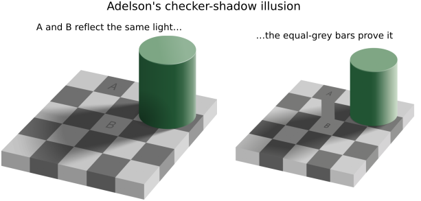
The canonical demonstration is Adelson's checker-shadow illusion (Figure 2.3.3): two checkerboard squares of identical pixel luminance look dramatically different — one "white in shadow," one "black in light" — because the brain infers the cast shadow and discounts it. Retinex (Land & McCann 1971) models exactly this computation: treat slow spatial gradients as illumination and sharp edges as reflectance changes, then integrate the edges back up to recover lightness. The same idea reappears as intrinsic images (splitting a photo into a reflectance layer and a shading layer) and, in the darkroom, as the craft of dodging and burning — locally cheating the illuminant that the eye is trying so hard to discount.

It is worth asking why the visual system goes to this trouble, and the answer is ecological. What matters for survival is the material world, not the light on it: whether that shape in the grass is a predator, whether that fruit is ripe enough to eat, whether the path ahead is dry stone or wet rock. Those are facts about reflectance, the fixed identity of surfaces, and they hold whether the sun is high or low and whether you stand in shade or glare. The illumination is a nuisance variable, the thing that swings from dawn to noon to dusk and from sun to cloud while the objects themselves do not change. An animal that tracked raw luminance would see the world lurch every time a cloud passed; an animal that recovers reflectance sees stable objects it can recognize and act on. So the brain is built to be invariant to the illuminant, to divide out the multiplicative factor and keep the surface term. We rarely need to know how much light there is; we need to know what the things around us are.

This same preference for reflectance has a practical echo in how photographers set exposure. Because what we ultimately want on the page is the surface and not the light that happened to fall on it, one can choose exposure from the incoming illumination rather than from the light coming off the subject. An incident-light meter does exactly this, with a translucent dome held at the subject and pointed back at the camera: it reads the light arriving while never seeing the subject's own tone. A grey card of known reflectance (the standard 18%), placed in the same light and metered in the subject's stead, does the same job with any ordinary reflected meter. Either way the exposure is pinned to the illumination alone, so the camera divides out that multiplicative factor much as the eye does and renders a surface to the same tone whether it sat in sun or shade (see Exposure).

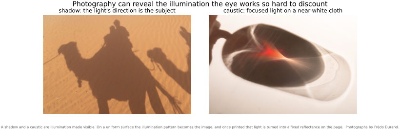
And yet the photographer sometimes wants the opposite. If the eye works so hard to divide the illuminant out and see through to the surface, one of the quiet magics of photography is to put the light back on stage, letting a raking low sun, a cast shadow, a shaft through a window, or the caustic thrown by a glass become the subject itself (Figure 2.3.4). Part of how a photograph pulls this off is that it turns illumination into reflectance. The shadow of a camel and its riders is only a pattern of light and shade on the sand, yet in the frame it reads as a solid shape. The caustic is pure focused light on a nearly white cloth, and because the cloth's reflectance is close to uniform, what the paper records is the illumination itself. Printed, that light becomes ink on the page, a fixed reflectance the viewer's eye will now dutifully discount all over again. The camera and the print quietly launder illumination into surface, which is exactly why a photograph can show us the very light our visual system spends its whole effort trying not to see.

2.3.3 Color constancy🔗⧉

Discounting the illuminant🔗⧉

Color constancy is the chromatic twin of lightness constancy. We perceive an object's intrinsic surface color — its spectral reflectance — despite large swings in the illuminant. A white shirt reads as white under noon daylight, under a warm tungsten lamp, and in cool blue shade, even though the spectra reaching the eye in those three cases differ enormously. Once again the brain discounts the illuminant: it estimates the color of the light and effectively divides it out, so the surface reads consistently. And once again this is the illuminant × reflectance inversion — ill-posed, solved with assumptions, such as "the average of the whole scene is roughly gray" or "the brightest patch is white."

A key biological mechanism is von Kries adaptation: an independent gain on each cone type (L, M, S) that rescales each channel to the prevailing light (Figure 2.3.5). It is beautifully simple — three multipliers — and it is the direct biological ancestor of a camera's white balance. It is also not perfect: some cast lingers, spatial and contextual cues fill the rest, and memory colors (we know bananas are yellow and grass is green) bias the result.

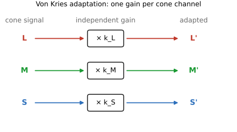
This whole process is the biological counterpart of white balance (next chapter): the camera's automatic white balance algorithm must compute, by gray-world, bright-pixel, Retinex, or Bayesian (Freeman & Brainard) heuristics, what our visual system does for free.

Constancy is not unconditional, and it degrades exactly where the machinery runs out of light. In dim scenes the cone signals grow noisy and the rods take over, and rod vision is colorblind. As the light falls toward twilight the world desaturates and shifts blue (the Purkinje shift), and below a fraction of a lux human color vision effectively stops, which is why a moonlit landscape reads as silver rather than green. Constancy also leans on cues that the dark removes: with few bright surfaces, weak specular highlights, and little inter-reflection, the visual system has almost nothing to estimate the illuminant from, so its guess drifts. This is not a side note for photography but part of its reason for being. The regime where our own constancy fails, low light, is precisely where a camera's computational white balance has to work hardest, and Google's Night Sight (Liba et al. 2019) trained a learned low-light white-balance model for exactly this reason: at around 0.3 lux there is no reliable cue and no human intuition left to copy.

Failure of color constancy when viewing photographs🔗⧉

Color constancy is an inference from cues, and it is only ever as good as the cues available. Maloney's analysis of the cues to the illuminant (Maloney 1999) makes the point sharply: the visual system must identify things like specular highlights and the brightest surface in order to estimate the light, and if it misreads one (mistaking a highlight for a surface's own color, say), constancy fails in a striking and predictable way. Kraft and Brainard (Kraft & Brainard 1999) turned this into an experiment, silencing individual cues one at a time in a real, nearly natural scene (local contrast, the brightest surface, the specular highlights) and watching constancy get progressively worse as each cue was removed. Constancy is not a fixed reflex; it is a cue-driven estimate that fades smoothly as the scene is impoverished.

A photograph is impoverished in exactly this sense, and it carries an extra problem all its own. A picture is two things at once: a flat object lying in your room under your room's light, and a window onto a depicted scene under some other light. Those two readings supply conflicting illuminant cues, the dual-code structure of picture perception (Mausfeld 2003 (dual code)). Faced with the conflict, the visual system adapts mostly to the display or print and its surround, not to the illuminant inside the picture. This is the working assumption of every color-appearance model, CIECAM and its media-relative rendering intent (Fairchild, Color Appearance Models): appearance is driven by the viewing condition's white point, surround, and luminance, not by the depicted scene's. And because adaptation is incomplete and mixed (the viewer is adapted partly to the ambient room and partly to the image's own white, a weighted compromise: the D-factor in CIECAM, Hunt's incomplete adaptation), a photograph shot under tungsten still looks orange even though a tungsten-lit room would not. That single fact is the mechanistic reason automatic white balance has to exist.

The experimental record agrees that constancy is poor on displayed images. Foster's review (Foster 2011) is candid that constancy is typically far from perfect, often only 20 to 60 percent by common measures, and Brainard's Bayesian model of human constancy (Brainard et al. 2006 (Bayesian human constancy)) explicitly reports viewing conditions in which observers' achromatic settings fall closer to the no-constancy prediction than to full constancy. Foster's later work on relational constancy (Foster 2023 (relational constancy)) shows the failure directly on screens: observers viewing pairs of scene images systematically misidentify an illuminant-corrected image as an illuminant change, with the errors growing as the cone-excitation ratios deviate. The estimate is also prior-driven, so it fails when the light is unusual: Delahunt and Brainard (Delahunt & Brainard 2004) found constancy markedly better for daylight-locus illuminant changes than for off-locus ones, the same reason constancy collapses almost entirely under a sodium street lamp, and the same statistical inference an automatic white balance is really performing.

Put together, the synthesis is clean and load-bearing. Constancy is good in rich, real, immersive scenes and poor in cue-impoverished ones. A photograph is cue-impoverished and embedded in a conflicting illuminant context, so the viewer adapts largely to the display and its surround rather than to the depicted illuminant. That is precisely why a camera must perform white balance computationally: the ISP is substituting for a constancy mechanism that the viewer, looking at a picture, can no longer run. The eye's failure at constancy on images is not a curiosity, it is the reason a whole stage of the pipeline has to exist.

This failure runs deeper than a nuisance, because it makes color technology genuinely hard, and it sharpens what the goal of color reproduction even is. A camera measures the spectrum that actually reaches it, or rather its three-filter projection of that spectrum: cone-like responses to the product reflectance × current illuminant. But that product is not what we want to reproduce. Because the viewer of the print will not run constancy and discount the depicted light, faithful reproduction has to deliver the cone responses the same scene would have produced under a neutral (canonical) illuminant, the colors the surfaces "really" are, stripped of the accidental light. Reaching that target means undoing the multiplication: dividing the measured product by an illuminant we never measured and must estimate. That is an ill-posed factorization of one measured spectrum into two unknowns, reflectance and illuminant, at every pixel, exactly the kind of separation taken up in Imaging as an inverse problem (§2.15). And it is hardest of all under a spiky illuminant (a fluorescent tube, a white LED, a sodium lamp), whose few narrow peaks sample the reflectances at only a handful of wavelengths, so the missing spectral information cannot be recovered and two surfaces a smooth daylight would have separated collapse together (the illuminant-metamerism trap of Perceptual color and trichromatic vision). The eye's own constancy hides this difficulty from us in the world; a camera, preparing a picture to be seen under yet another light, has to confront the factorization head-on.

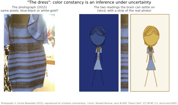
Even when the visual system does try to run constancy on a photograph, the ambiguity can leave it genuinely undecided, and different viewers commit to different priors. That is the whole story of "the dress" Lafer-Sousa et al. 2015 (Figure 2.3.6). The viral 2015 photograph shows identical pixels that some people see as blue-and-black and others as white-and-gold, because each viewer's brain silently guesses the illuminant, cool daylight versus warm indoor light, and divides it out differently. The dress is the perfect proof that color constancy is an inference under uncertainty, not a measurement: the visual system commits to a prior, and different people commit to different priors. A camera faces the exact same ill-posed guess.

2.3.4 Contrast🔗⧉

If there is one mathematical theme to perception, it is that vision cares about ratios, not absolute values — a direct consequence of operating in a multiplicative world under wildly varying light. A step from luminance 1 to 2 looks like the same step as 100 to 200: in both cases the light doubled, and doubling is what the eye registers. This automatically discounts the multiplicative effect of the illuminant (a brighter light scales everything equally, leaving ratios untouched) and it is the direct perceptual reason we will later encode images in gamma or log — to spend code values where the eye actually looks.

This is the multiplicative world of L2.6 once more, now seen from the perceptual side. The image is illumination × reflectance, so a ratio of two nearby image values divides the shared illumination out (it cancels top and bottom) and leaves a ratio of pure reflectances. Contrast, being a ratio, is therefore a reflectance quantity almost by construction: it is what survives when the illuminant is factored away. So the eye's insistence on ratios is not an arbitrary quirk but the same illuminant-discounting we just saw in lightness and color constancy, built this time into the very currency of vision. It is also why a logarithmic encoding is so natural here: in the log domain a ratio becomes a difference and the multiplicative illuminant becomes an additive offset that the visual system, and later the pipeline, can simply subtract off.

Quantitatively, this is Weber's law: the just-noticeable increment in intensity is roughly a constant fraction of the background, $\Delta I / I \approx \text{const}$. The smallest brightness change you can detect grows in proportion to the brightness you are already looking at — the signature of a logarithmic-ish response. For describing the contrast of a pattern (rather than a single increment) the standard measure is Michelson contrast,

a normalized, level-independent ratio. Contrast also depends on context: a gray patch looks lighter on a dark surround and darker on a light one (simultaneous contrast), and the Adelson checker-shadow illusion is the same effect dressed up. Ratios, not absolutes, all the way down.

2.3.5 Spatial vision🔗⧉

How fine a pattern can we resolve, and how does sensitivity vary with the scale of the detail? Visual acuity — the familiar eye-chart measure — sets the finest line spacing we can make out, but it is only the high-frequency tail of a richer story.

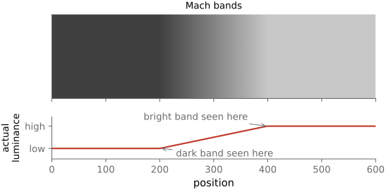
Two low-level mechanisms shape spatial vision. Lateral inhibition wires each retinal cell to subtract a weighted average of its neighbors, producing center–surround receptive fields that respond to local contrast rather than absolute level — an edge enhancer built into the retina. Its signature is Mach bands (Figure 2.3.7): at a ramp between two gray levels you see illusory bright and dark bands hugging the edges, the center–surround filter overshooting. The same wiring underlies simultaneous contrast from the previous section.

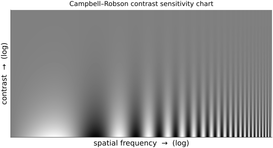
The full description is the contrast sensitivity function (CSF), measured by psychophysics: show the observer sine-wave gratings of varying spatial frequency and contrast, ask "do you see a grating?", and trace the threshold. The CSF turns out to be band-pass — sensitivity peaks at intermediate spatial frequencies and falls off at both very coarse and very fine scales (the high-frequency cutoff is acuity).

This experiment can be reproduced directly (Figure 2.3.8). In the Campbell–Robson chart Campbell & Robson 1968, spatial frequency rises to the right and contrast rises downward, the same contrast range in every column, yet the height at which the stripes fade into flat gray is an inverted U, not a level line. The visibility boundary traces the observer's contrast sensitivity function. And because the CSF is measured in cycles per degree of visual angle, the boundary moves with viewing distance: step back and the fine bars on the right vanish first.

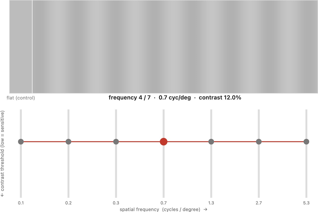
You can also run the experiment the way a vision scientist would — by adjustment, one frequency at a time (Figure 2.3.9). Seven sliders, one per spatial frequency, each set the contrast of its grating; lower each until the stripes just vanish, and the slider tops draw your threshold curve point by point — the U-shaped dual of the inverted-U sensitivity. The demo takes the display seriously, because a CSF measurement is exactly where naïve rendering lies: the grating is built in linear luminance, sRGB-encoded for the screen, and ordered-dithered so 8-bit quantization cannot fake or hide a near-threshold grating, with a zero-contrast flat patch as a control.

A computational model. The luminance CSF is not just a curve to look at — it has a closed form you can evaluate, which is what lets it drive real algorithms. The classic fit is Mannos–Sakrison (Mannos & Sakrison 1974),

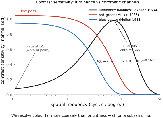
with $f$ in cycles per degree of visual angle: a band-pass curve peaking near 8 cpd, finite at DC (≈5 % of peak), and falling toward the ~50–60 cpd acuity limit. Because $f$ is per degree, any use of the model must first convert image cycles-per-pixel to cycles-per-degree using the viewing distance and display resolution — the same dependence the Campbell–Robson demo makes tangible. Barten's more complete model (Barten 1999) adds the dependence on luminance and stimulus size and is what underlies the DICOM medical-display standard and the SMPTE-2084 (PQ) HDR transfer curve. Used as a perceptual weighting, $A(f)$ is exactly what tells a codec or quality metric which spatial frequencies to spend bits on — directly behind JPEG's quantization tables and metrics like SSIM's successors.

Crucially, there is not one CSF but three, and they differ dramatically (Figure 2.3.10): the chromatic CSFs — for the red–green and blue–yellow opponent channels — cut off at far lower spatial frequency than the luminance CSF. We resolve color far more coarsely than brightness. These are not hand-waving sketches: the luminance CSF has well-known quantitative models — the closed-form Mannos–Sakrison fit $A(f)=2.6\,(0.0192+0.114f)\,e^{-(0.114f)^{1.1}}$ (Mannos & Sakrison 1974) used in image-quality metrics, and Barten's more complete model (Barten 1999) that underlies the DICOM display standard and the SMPTE-2084 (PQ) HDR curve — while the chromatic channels follow Mullen's measured low-pass functions (Mullen 1985). One detail the models insist on: the luminance CSF is band-pass but its low-frequency sensitivity does not fall to zero — a large uniform field still has finite contrast sensitivity (≈5 % of the peak), which is why a slow gradient across the whole frame is still visible.

This yields one of the most consequential demonstrations in the book. Convert an image to an opponent (luma/chroma) space and blur the chroma channels heavily — the picture still looks sharp. Blur the luminance channel instead and it falls apart. The eye simply does not resolve fine color. This is the empirical licence for chroma subsampling in JPEG and video (store color at half or quarter resolution), and a clean confirmation of the opponent model and its three separate CSFs.

It is worth pausing on why the gap exists, because the answer ties this section back to the opponent recoding several sections ago. The coarseness of color vision is not a property of the cones — it is built by the retinal wiring. Luminance is the sum $L+M$, carried by dense, small-field pathways with tight center–surround receptive fields, so it has high spatial bandwidth. Chrominance is carried by the opponent differences $L-M$ and $S-(L+M)$, and those differences are computed in the retina and LGN (the stage-2 opponent recoding, L2.14) by pooling cones over larger regions — and the blue–yellow channel is further starved by the sparse S-cone mosaic (almost none in the central fovea, from the anatomy section). Spatial pooling of a difference is exactly a low-pass operation. So the three separate CSFs of L2.15 are not an accident: they are the direct spatial signature of the in-retina opponent transform. The eye builds detail from a dense sum and color from sparse, pooled differences — and image compression, when it splits luma from chroma and subsamples the chroma, is simply re-discovering the eye's own retinal architecture.

2.3.6 Temporal vision🔗⧉

The visual system trades some spatial resolution for temporal resolution. Just as there is a contrast sensitivity function over spatial frequency, there is a temporal CSF over flicker frequency, and it too is band-pass. Above a critical flicker-fusion frequency — roughly 50–60 Hz in bright light, lower in dim — a flickering source fuses into a steady one. This is why displays and projectors refresh fast enough to look continuous, and why old cathode-ray-tube screens and fluorescent tubes could be seen to flicker in peripheral vision (the periphery, rod-rich, has a higher fusion frequency) even when the center of gaze saw them as steady.

A computational model. Like the spatial CSF, the temporal CSF has quantitative forms. A workable closed model treats flicker sensitivity as a band-pass filter over temporal frequency $\omega$ (Hz), built from a fast transient channel and a slower sustained one — e.g. the difference of two low-pass stages, $S(\omega) \propto \big|\,(1+i\,2\pi\omega\tau_1)^{-n_1} - \zeta\,(1+i\,2\pi\omega\tau_2)^{-n_2}\big|$ (the linear-filter form due to Watson Watson 1986) — which peaks near 8–10 Hz and rolls off to the flicker-fusion limit. But spatial and temporal sensitivity are not separable, and the modern, unified treatment is Mantiuk and colleagues' stelaCSF (Mantiuk et al. 2022): a single parametric model that gives contrast sensitivity $S$ as a joint function of spatial frequency, temporal frequency, luminance, eccentricity, and stimulus area, fit to a large pooled psychophysical dataset and released as open code. Its color extension castleCSF (Ashraf & Mantiuk 2024) adds the chromatic (red–green and yellow–violet) directions to the same unified surface.

It is worth writing castleCSF out, because it shows how much of "what the eye can see" is now captured by one explicit formula. The model gives the sensitivity $S$ (the reciprocal of the threshold contrast) for each of three color-opponent channels $c\in\{\text{ach},\,\text{rg},\,\text{yv}\}$ — achromatic, red–green, yellow–violet — as a function of six stimulus variables: spatial frequency $\rho$ (cpd), temporal frequency $\omega$ (Hz), background luminance $L$ (cd m$^{-2}$), retinal eccentricity $e$ (deg), stimulus area $A$ (deg$^2$), and the channel $c$ itself. The achromatic channel is stelaCSF; the two chromatic channels are the castle extension. For each channel the sensitivity factors into one term per dependence:

and each factor has a measured closed form:

• Spatio-temporal $M_c(\rho,\omega)$ — deliberately not separable in $\rho$ and $\omega$; it is built from a sustained and a transient temporal channel, each gating a spatial response, so a static grating leans on the sustained channel and flicker on the transient one (this is precisely why high spatial detail wants a still image while fast motion tolerates blur).
• Luminance $G_c(L)$ — peak sensitivity climbs with light along the two classic regimes: deVries–Rose ($S\propto\sqrt{L}$, photon-noise-limited) in the dark, flattening into Weber behavior ($S$ roughly constant) in daylight.
• Area $P_c(A,\rho)$ — sensitivity grows as the grating covers more of the field (probability / contrast summation over cycles, Rovamo's law), saturating once enough cycles are present.
• Eccentricity $E_c(e,\rho)$ — sensitivity falls away from the fovea, and falls faster at high spatial frequency — the quantitative basis of foveated rendering.

The exact fitted constants (the peak sensitivities $S^{\text{peak}}_c$, the sustained/transient time constants, the luminance and eccentricity rates) come from jointly fitting all of these to a large pooled psychophysical dataset, and are distributed as open reference code [@mantiuk-stelacsf-2022; @ashraf-castlecsf-2024]. The point is not the specific numbers but that they exist: a single evaluable function now predicts the visibility of any grating — of any color, at any speed, brightness, size, and position in the visual field — which is exactly the front end every modern HDR / video quality metric and display-engineering pipeline runs on.

Closely related is apparent motion — the phi phenomenon — by which a sequence of still frames reads as continuous movement; together with persistence of vision it is what makes cinema and video possible (→ Motion/Video). Temporal vision also has its own adaptation (the seconds-to-minutes light/dark adaptation of the previous section) and is shaped by the eye's own constant motion — the saccades and microsaccades of the next section. Computation exploits all of this: choosing frame rates, capturing flicker-free under pulsed lighting, and video magnification (amplifying tiny, normally invisible temporal changes — a color or motion signal too small to notice — covered in Motion/Video).

2.3.7 Attention and eye movements🔗⧉

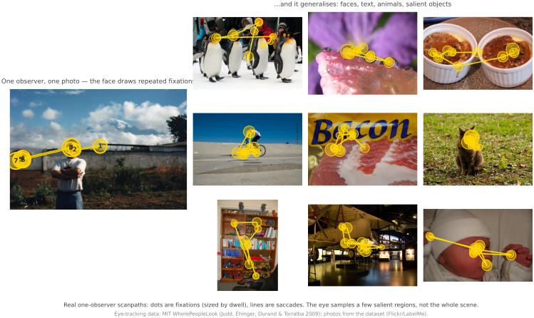
Vision is not a uniform snapshot. Only the fovea sees in high resolution, so the eye samples a scene through a rapid sequence of fixations punctuated by saccades — fast, ballistic jumps that re-aim the fovea — with smooth pursuit to track moving targets. We feel as though the whole scene is sharp, but that is another construction: the brain stitches together a few high-resolution glimpses and fills in the rest. A record of where the eye lands over time is a scanpath (Figure 2.3.11), and it is far from random — it is drawn to salient regions (faces, motion, high contrast, the unexpected).

This pattern generalizes across images: across very different photographs the eye keeps going to the informative places (Figure 2.3.11, right).

What draws the eye — saliency — can be modeled, and modern saliency and gaze-prediction models are learned with machine learning (→ the saliency / gaze-prediction material in the Machine learning part). Saliency in turn feeds content-aware image operations: where can we crop or retarget an image without disturbing what the viewer will actually look at? That is the link to auto-cropping and seam carving later in the book.

Long before any of this was measured, artists were doing it by hand. Guiding the viewer's attention — controlling where the eye goes, and in what order — is one of the central things a painter, photographer, or cinematographer does, and it is precisely what composition is for: leading lines, contrast and brightness, selective focus, color accents, framing, and the placement of the subject all steer the gaze toward what matters and away from what doesn't. The scanpath and saliency map are simply the empirical, measurable face of a craft that has always been about directing attention (→ the composition tactics in the Human factors part).

2.3.8 The visual system makes things up🔗⧉

We just said the feeling of a sharp, complete scene is a construction. It is worth dwelling on how radical that construction is, because it undercuts an assumption that quietly shapes how people think about photographs: that seeing is like taking a picture, a faithful, detailed, all-at-once recording of what is in front of you. It is not. What actually reaches the brain is a tiny sliver of high-resolution color from the fovea (a patch spanning only a degree or two, a fraction of a percent of the visual field), surrounded by a vast low-resolution periphery that is poor at color and cannot resolve a face or a word, degraded further by crowding (nearby clutter jams recognition), punched through by a blind spot where the optic nerve leaves, and blanked briefly on every saccade (saccadic suppression) several times a second. Out of that ragged, mostly-empty input the brain manufactures the seamless, stable, fully-detailed world you seem to see. Aaron Hertzmann calls the result the illusion of awareness (Hertzmann 2024 (blog: illusion of awareness)): we are confidently certain we perceive everything in front of us, and we are wrong.

The evidence is a handful of demonstrations that are genuinely startling the first time you meet them. In inattentional blindness, an observer told to attend to one thing fails to notice something enormous and obvious in plain sight; the canonical version is Simons and Chabris's invisible gorilla, in which viewers counting basketball passes miss a person in a gorilla suit walking through the middle of the scene and thumping their chest (Simons & Chabris 1999 (invisible gorilla)). In change blindness, large changes between two views, or slow changes over time, go completely unnoticed when they fall outside the current focus of attention (Rensink, O'Regan & Clark 1997 (change blindness)); in the "door study," experimenters swapped the very person a subject was mid-conversation with, and about half the subjects never noticed. These are not edge cases or lab tricks. Wolfe, Kosovicheva and Wolfe call the everyday version normal blindness: looking without seeing is the default condition of vision, not a malfunction (Wolfe et al. 2022 (normal blindness)). And the periphery we assume is full of detail is, when measured, a statistical summary rather than a picture, which is why you cannot read this sentence out of the corner of your eye (Rosenholtz 2016 (peripheral vision)).

Why this matters for a book about photographs. First, it dissolves the intuition that a photograph is objective because the eye is a camera. The eye is not a camera, and the experience of vision is already an active, selective, largely invented reconstruction, so a photograph is not a degraded copy of some perfect inner image (a thread picked up in Photographs are usually not passive objective recordings). Second, it explains why so many of the perceptual shortcuts this book relies on actually work. Tone mapping, lossy compression, denoising, and content-aware retargeting can all discard or alter enormous amounts of the signal precisely because the viewer was never registering most of it: the eye samples a few salient points (the scanpath and saliency of the previous section) and the brain fills in the rest. A visual system that demanded a perfect internal picture would be impossible to fool; a visual system that makes things up is one you can economize against, which is much of what computational photography quietly does.