💬Comments welcome. To leave a note, select any text and click the note / highlight button that pops up — or open the panel with the tab at the top-right (‹). Notes are visible only inside our private review group.
PS1 implements brightness/contrast, gamma, and white balance as point operations. → Problem sets (appendix).
The simplest image-editing operations are independent at each pixel: each output pixel depends only on the value of the input pixel at the very same spot, with no reference to its neighbors or to where it sits. These are point operations, and they cover a remarkable fraction of the edits photographers actually make: exposure, brightness, contrast, levels, freehand tone curves, gamma, saturation and vibrance, white balance, and the lookup tables that bake them in. This chapter is about that whole family — what they can and cannot do, and the single question that decides whether each is done right or wrong: the numerical space it acts in.
Two framing cautions before the toolkit. First, these sliders are not independent: brightness, exposure, contrast, levels, and the tone curve all bend the same transfer line, so they overlap and partly undo one another; the general tone curve at the end of the chapter literally subsumes the rest, and any given look can be reached several ways. Second, they are not all equally meaningful: a few are objective, radiometric operations faithful to how light behaves (exposure is a multiply in linear light), while most are stylistic — brightness, contrast, the S-curve, saturation — with no single physically correct form, only a choice of space and taste. Knowing which kind you are using tells you whether "which space?" has a right answer (radiometric: yes) or merely a pleasant one (stylistic: pick the look).
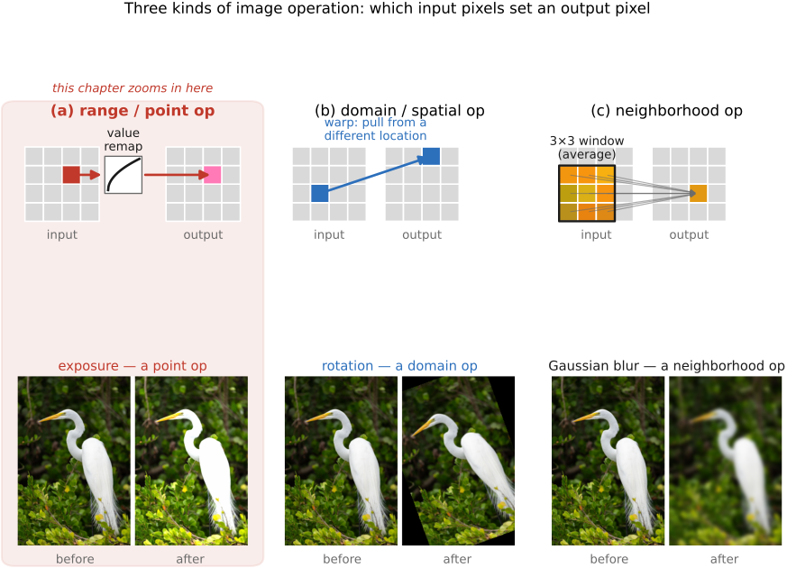
Before zooming in, it pays to sort every image operation into one of three families, according to what each output pixel is allowed to read (Figure 4.4.1). Recall that an image is a function over a 2-D domain — the grid of positions (x, y) — whose values live in a range, here color (we set this up in Image representation). The three families are precisely the three ways an operation can touch the domain and the range.
A point operation touches the range only. The output pixel depends solely on the input pixel's value at the same location, and one and the same rule is used everywhere:
There is a single input-to-output curve f, applied identically at every pixel. In words: read a pixel's value, find where that value lands on the curve, write the answer back — no neighbors consulted, nothing moved. Brightness, contrast, exposure, gamma, and lookup tables are all point operations, and we begin here because they are the simplest to reason about and the cheapest to run.
A domain operation is the mirror image: it relocates pixels without changing their colors, so the output pixel is copied from a different input location, $I_\text{out}(x, y) = I_\text{in}(x', y')$ for some remapped (x', y'). Resizing, rotating, warping, and lens-distortion correction live here; they are the subject of the resampling chapter.
A neighborhood operation sits in between: the output pixel is computed from a whole window of input pixels around the same spot. Blur averages a pixel with its neighbors; sharpening, edge detection, and the bilateral filter all read a neighborhood. Those get their own chapter on convolution.
Figure 4.4.1.The three families of image operation, sorted by what each output pixel may read. Point / range (left): the output depends only on the input pixel's value at the same location — one curve applied everywhere (exposure, contrast, lookup tables). Domain (center): pixels are relocated, their colors unchanged (resize, rotate, warp). Neighborhood (right): the output is computed from a window of nearby input pixels (blur, sharpen, bilateral). This chapter is the left column.
Everything below stays in the left column. One convenience keeps the discussion clean: a point operation acts on a single number, so we develop it on a grayscale value L and write the curve $L_\text{out} = f(L_\text{in})$; for a color image the same curve is applied independently to each of the R, G, B channels — unless we say otherwise. (Saturation, near the end, is the one genuine exception that couples the channels.)
Since a point operation is just one curve f applied to every pixel, the curve is the operation, and photo editors hand it to you directly: the curves tool plots input value across the horizontal axis, output value up the vertical, and lets you bend the line by hand. The "do nothing" case — leave every value untouched — is the 45° diagonal. Everything in this chapter is some way of bending that diagonal: lift it to brighten, steepen it to add contrast, pin its ends to set black and white points, or just drag it freehand.
Controlling that mapping is not a digital invention. Photography has always been the craft of deciding how scene radiance becomes printed tone — film stock, exposure, development, paper grade, and the enlarger all shape it — and the digital tone curve is the most direct handle on the same problem. There is, though, one question we must answer before we bend anything, and it runs through the whole chapter: in which numerical space does the curve act?
Sidebar — the Zone System
Ansel Adams and Fred Archer's Zone System is the most disciplined version of that craft and a fine mental model for the whole chapter. It carves the tonal range into eleven zones, Zone 0 (pure black) through Zone X (pure white), each a stop apart, with Zone V the mid-gray a light meter reads. The photographer previsualizes which scene tone should land in which zone, then works the mapping in two stages: scene → negative (exposure and the choice of film fix where the shadows fall; development time governs how far the highlights stretch) and negative → print (paper grade and local dodging and burning place each tone, sometimes region by region). The digital descendants are exactly the tools below — exposure sets where the tones fall, the tone curve reshapes the mapping globally, and masked local edits are the dodging and burning. This is also where the book's recurring theme of separating measurement from rendering comes from, and we return to it when local tone mapping arrives.
The same image can be stored as linear-light values (proportional to the physical radiance the sensor measured), as gamma/sRGB-encoded values (the perceptually spaced numbers a PNG actually holds), or as log values (handy when the range is enormous). We met these encodings in Image representation; here they stop being a storage detail and start changing the result. Apply the very same arithmetic in linear light versus in sRGB and you get visibly different pixels — so every operation below carries a note about the space it belongs in.
💡 Big lesson (L2.19) — additive vs. multiplicative → choice of encoding
The single most useful question to ask of any tonal operation is whether it is fundamentally additive or multiplicative, because the answer dictates the right encoding. A multiplicative change — scaling the light, the way exposure does — is natural in linear light (and becomes a plain addition in log). An additive change in display space — brightness, a fixed offset — lifts every value by the same amount, regardless of how much light there was to begin with. Light itself is multiplicative (double the photons, double the radiance), and perception is closer to multiplicative too: contrast is about ratios, not differences — the step from 1 to 2 looks like the step from 100 to 200. That is why so much of imaging prefers linear or log over a naive offset. Keep asking "additive or multiplicative?" and the choice of space usually answers itself.
Exposure is the workhorse, and it has a clean physical meaning. On the camera, changing the exposure — a longer shutter, a wider aperture, a higher ISO — multiplies the light recorded at every pixel by one common factor (we develop the controls themselves in the sensor chapter). Double the exposure and you double the radiance: a purely multiplicative effect, whose natural unit is the photographic stop, one stop being a factor of two. An adjustment of s stops therefore multiplies the linear-light value by $2^s$:
$$ L_\text{out} = 2^{s}\, L_\text{in}. $$
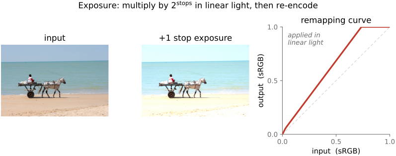
Plotted in display space the +1-stop curve bows upward above the diagonal, lifting the shadows generously and flattening as it nears the top; whatever it pushes past 1 is clipped to white and gone for good (Figure 4.4.3). That is the real cost of brightening: blown highlights do not come back.
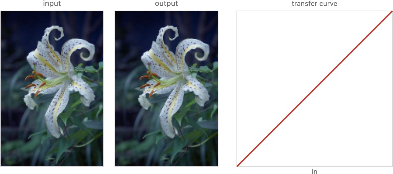
Figure 4.4.2.A point-operation playground. Every pixel is mapped through the same function, independent of its neighbors: exposure, brightness, contrast, gamma, saturation, threshold, and invert all compose into the single input→output transfer curve shown at right. Adjust the controls (or load your own image) to watch the curve and the result change together — the rest of this section unpacks these one at a time.Figure 4.4.3.Exposure as a multiply in linear light. Left, the input. Center, the same photo at +1 stop (×2 in linear light) — brighter throughout, with the brightest highlights clipped to white. Right, the transfer curve $L_\text{out} = 2^{s} L_\text{in}$ drawn in display (sRGB) space: it bows above the 45° diagonal, lifting the shadows strongly and flattening into the ceiling at 1. The 45° diagonal (no change) is shown for reference.
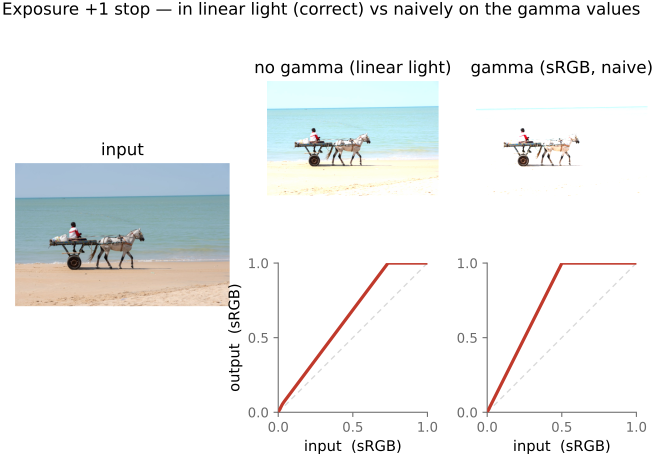
The "in linear light" qualifier is not pedantry. It marks the difference between a correct exposure change and a wrong one. The library makes the distinction concrete: imageops.exposure(img, stops) decodes to linear light, multiplies, then re-encodes; ask it for the naive version instead and it multiplies the gamma-encoded numbers directly, which is exactly what happens when you forget to linearize. The two part ways sharply, and the next figure is devoted to showing how.
💡 Big lesson (L4.2) — exposure scales linear light (a multiply) or shifts log values (an add)
Changing exposure is a multiplication of linearly-encoded values ($L_\text{out}=k\,L_\text{in}$, with $k=2^{s}$ for $s$ stops) — equivalently an addition in log/stops ($\log L \mapsto \log L + \log k$). In gamma-encoded data it is neither, so the right move is to convert to linear (or log), apply, convert back. If you must work in place, the exact gamma-space map is still a multiply, but by $k^{1/\gamma}$ rather than $k$: $L_\text{out}=k^{1/\gamma}\,L_\text{in}$ — the kind of off-by-a-gamma error that bites silently. This is the cleanest case of L23, "do the physics in linear light, apply gamma last."
Figure 4.4.4.Why the space matters for exposure. The same "+1 stop" done two ways. Top, the correct way — multiply in linear light (decode → ×2 → re-encode): tones brighten smoothly and in proportion. Bottom, the naive way — multiply the gamma/sRGB numbers directly: the curve is a straight ramp of slope 2 that clips everything above input ½ to white, blowing out the entire upper half of the tonal range. Same intended edit, very different pixels — exposure belongs in linear light.
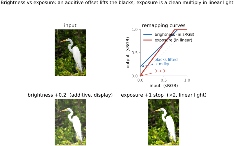
It is tempting to think a "brightness" slider does the same job, but it does something subtly worse. Brightness is an additive offset: it adds the same constant b to every value,
$$ L_\text{out} = L_\text{in} + b, $$
which slides the whole transfer line straight up by b (a parallel shift, intercept b). The trouble is what it does to black. Exposure keeps black at black — multiply zero by anything and it stays zero — but brightness lifts true black off the floor to b, so the darkest tones turn into a flat, milky gray and the shadows look fogged (Figure 4.4.5). For that reason we generally recommend against brightness and for exposure: exposure is the more radiometric control, faithful to how light actually scales, whereas brightness survives mostly as a legacy slider or a quick-and-dirty shadow lift.
Figure 4.4.5.Brightness (additive) versus exposure (multiplicative). Left, the input. Center, two outputs matched to lift the midtones by the same amount: brightness $L+b$ raises the blacks off zero, fogging the shadows into flat gray, while exposure $2^{s} L$ keeps black at black and scales in proportion. Right, both transfer curves — brightness is the diagonal shifted straight up (a parallel line, intercept b); exposure passes through the origin and fans upward. Only the multiplicative curve preserves true black.
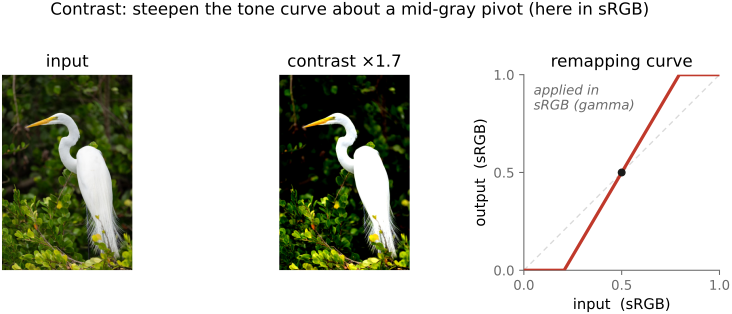
Where exposure moves all the tones the same way, contrast spreads them apart or pulls them together. The idea is to pick a pivot value — a mid-gray that stays put — and push every other value away from it (more contrast) or toward it (less). Values above the pivot get brighter, values below get darker, and the pivot itself never moves. As a curve, that is a straight line through the pivot whose slope is the contrast gain g:
$$ L_\text{out} = g\,(L_\text{in} - p) + p, $$
where p is the pivot. Read it as: measure how far a value sits from the pivot, scale that distance by the gain, add it back. A gain above 1 steepens the line and raises contrast; a gain below 1 flattens it and lowers contrast. The steeper the line, the sooner it slams into the floor at 0 and the ceiling at 1 — so strong contrast clips both shadows and highlights (Figure 4.4.6).
💡 Big lesson (L4.3) — contrast is a pivot: choose what stays put
A contrast change rotates values about a chosen pivot: $L_\text{out} = p + g\,(L_\text{in}-p)$. The pivot $p$ is exactly what is left unchanged, and it also decides whether the picture gets brighter or darker overall — a high pivot pulls most of the image down (darkening), a low pivot pushes it up (brightening). Unlike exposure, contrast is not radiometrically meaningful — it is a stylistic stretch — so the encoding matters less (no single space is "correct"); what matters is a sensible pivot, and the sensible pivot does depend on the space: roughly 18% mid-gray in linear light, the numeric midpoint in gamma or log. Pick the pivot deliberately — it is the whole character of the operation.
Sidebar — 18% gray, and the space it lives in
Where should the pivot sit? The photographer's answer is 18% gray — a mid-tone reflectance that light-meters are calibrated to and that the Zone System places in Zone V (developed in the tone-mapping chapter). The "18%" is a fraction of linear reflectance/luminance, not of a gamma-encoded number — which is why it lands near the middle of a gamma-encoded range ($0.18^{1/2.2}\approx 0.46$) but low in linear. Two practical consequences: a contrast pivot meant to hold the mid-tones should be 18% in linear light (or ≈0.46 if you steepen in gamma); and when you compute an image's "average tone" for auto-exposure or a gray-world white balance, do the averaging in linear light (where light adds), not on gamma values, or the mean is biased bright. We meet 18% again at exposure metering (the sensor chapter) and the Zone System (tone mapping).
Figure 4.4.6.Contrast as a steepening about a pivot. Left, the input; center, increased contrast (gain > 1) — shadows deepen, highlights brighten, midtones near the pivot barely move; right, the transfer curve, a straight line through the mid-gray pivot p whose slope is the gain. Steepening drives the line into the floor (0) and ceiling (1), clipping the darkest and lightest tones. The 45° diagonal (gain 1, no change) is shown for reference.
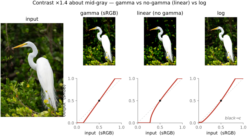
And here the recurring question bites hardest: in which space do we steepen? Unlike exposure, contrast has no single physically correct answer. It is a stylistic operation, and the choice of space changes its character outright (Figure 4.4.7). Steepen in sRGB/gamma (the default in most editors, and the library's default for imageops.contrast) and the pivot sits at a perceptual mid-gray, so the effect roughly tracks how the eye judges contrast. Steepen in linear light and the gain acts on physical radiance, which weights the highlights very differently and tends to look harsher, crushing the shadows. Steepen in log (a density-like space) and the operation becomes a uniform stretch in ratios, the gentlest on a wide range. None is wrong. They are three legitimate looks, and a good editor lets you choose. We flag the spread here and defer the full radiometric-versus-perceptual argument to the tone-mapping chapter, where it shapes the design of high dynamic range (HDR) operators.
Figure 4.4.7.The same contrast boost in three spaces. The identical gain about a mid-gray pivot, applied in sRGB/gamma (perceptual mid-gray — the usual editor behavior), in linear light (acting on physical radiance — harsher in the highlights, crushes the shadows), and in log/density (a uniform stretch in ratios — gentlest across a wide range). For the log version the black is clamped to a small ε to avoid log(0). Each panel shows the output and its transfer curve; the look differs because the pivot and the spacing of tones differ between spaces.
Sidebar — the S-curve
A straight contrast line clips abruptly the moment it touches 0 or 1. Photographers usually prefer a sigmoid (S-shaped) tone curve instead: steep through the midtones (where the eye is most sensitive) but easing gently into the shadows and highlights so the extremes roll off rather than clip. This is exactly the shape of film's response and of a camera's built-in "look," and it is the bridge both to the general tone curve below and to the tone-mapping operators of the next chapter.
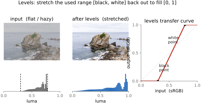
Most photographs do not use the full tonal range: the darkest pixel might sit at a murky 0.08, the brightest at a dull 0.9, leaving the image flat and hazy. The levels tool fixes this by stretching the used range back out to fill [0, 1]. You set a black point — the input value that should map to 0 — and a white point — the input value that should map to 1 — and everything between is stretched linearly across the full range; anything below the black point clips to black, anything above the white point clips to white. A third control, a mid-gray gamma slider, bends the curve between the two anchors to lift or lower the midtones without disturbing the endpoints.
The black point earns special mention because it does more than add snap. When unwanted light is added uniformly across the frame — a veiling glare from a dirty or flared lens, or atmospheric haze scattering light into every pixel — the effect is an additive pedestal that lifts the blacks off the floor (the same milky, fogged look brightness produces). Raising the black point subtracts that pedestal back off, restoring true black and the contrast the stray light washed out. That is a first, global taste of dehazing: haze is exactly an additive (and depth-dependent) veil, and the simplest correction is a black-point subtraction — the spatially-varying, physically-modeled version is the dark-channel and atmospheric-scattering work we take up in dehazing.
A word on space, since the chapter's throughline demands it: levels (like contrast) is a stylistic stretch with no single correct encoding, but the two endpoints behave differently. The black-point subtraction is physically an additive correction of stray light, so it is most defensible in linear light (where the veiling glare actually adds); the white-point stretch and the mid-gray gamma are perceptual adjustments usually done, like most editing, in gamma/sRGB. Most editors run levels in display space for responsiveness; just know that a black-point pull meant to remove haze is the one piece that strictly belongs in linear light.
Levels is the first edit on almost every image, and it is really a piecewise version of the curves we have already met — clip-and-stretch at the ends, a gamma bow in the middle (Figure 4.4.8). The natural way to set it is by eye on the histogram: pull the black point up to where the dark tones actually start, pull the white point down to where the bright tones end, and nudge the gamma until the midtones sit right. That makes the histogram — which earns its own short chapter next — the levels tool's constant companion.
Figure 4.4.8.Levels on a real photo. Left, the input — a flat, hazy coastal scene whose tones are bunched in the middle of the range, with no true black and a dull off-white that never reaches 1 (its luma histogram, below, is a narrow hump bounded by the black- and white-point markers). Center, after levels: the used range $[\text{black}, \text{white}]$ has been stretched out to fill $[0, 1]$, so the histogram spreads to both edges and the image gains contrast and snap. Right, the transfer curve — flat (clipped) below the black point, flat (clipped) at 1 above the white point, and a straight stretch between the two anchors (a mid-gray gamma would bow this middle segment).
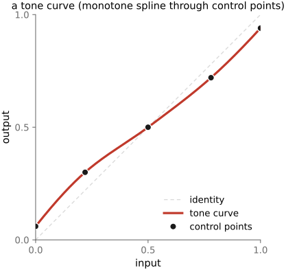
Exposure, contrast, and levels are all constrained shapes — a fan, a straight steepen, a clipped stretch. The most general point operation simply lets you draw the curve freehand: the tone curve tool gives you a handful of control points to drag wherever you please, and the editor threads a smooth interpolating curve through them (Figure 4.4.9). To keep the result sane, the curve is fit with a spline that is held monotone, never decreasing, so a brighter input can never produce a darker output. (A non-monotone tone curve would invert tones locally, which looks bizarre.) Catmull–Rom and monotone-cubic splines are the usual choices, the latter when the no-inversion guarantee must be exact.
Figure 4.4.9.The general tone curve. A few draggable control points (dots) are interpolated by a smooth monotone spline (solid) into an arbitrary transfer curve; the 45° identity is shown dashed. Because the spline is kept monotone — never decreasing — a brighter input never maps to a darker output, so tones cannot invert. This single freehand curve subsumes the exposure bow, the contrast steepen, and the levels stretch of the earlier figures.
Sidebar — splines (the math)
A spline fits a smooth curve through a set of control points (knots) $(x_i, y_i)$ by stitching together low-degree polynomial pieces — for our purposes one cubic per interval $[x_i, x_{i+1}]$, with the pieces joined for continuity. The cleanest way to write each piece is the cubic Hermite form. On $[x_i, x_{i+1}]$, set $t = \frac{x - x_i}{x_{i+1} - x_i} \in [0, 1]$ and write
The piece passes through $y_i$ at $t=0$ and $y_{i+1}$ at $t=1$ no matter what; the only free choice is the tangent (slope) $m_i$ at each knot — and that choice is what separates the schemes:
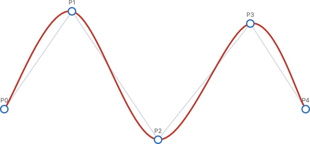
Catmull–Rom (interpolating, $C^1$): take the tangent as the centered difference $m_i = \frac{y_{i+1} - y_{i-1}}{x_{i+1} - x_{i-1}}$ — local and cheap, but it can overshoot between knots and so go non-monotone.
natural cubic ($C^2$): demand continuous second derivatives and minimize the total curvature $\int (p'')^2$; this couples all the knots into one tridiagonal linear system for the slopes — the smoothest fit, but it too can overshoot.
monotone cubic (Fritsch–Carlson): start from Hermite tangents, then clamp them so every segment is monotone. Write the secant slope $\Delta_i = \frac{y_{i+1} - y_i}{x_{i+1} - x_i}$; where a secant is flat ($\Delta_i = 0$) set the neighboring tangents to $0$, and otherwise keep $(\alpha, \beta) = (m_i/\Delta_i,\ m_{i+1}/\Delta_i)$ inside the circle $\alpha^2 + \beta^2 \le 9$. This guarantees no inversion — exactly the property a tone curve needs (brighter in $\Rightarrow$ brighter out), which is why it is the standard choice here.
B-splines are the approximating cousin: the curve follows a control polygon and need not pass through the knots — smoother and easy to keep monotone, at the cost of exact interpolation.
Sidebar — spline families (drag to compare)
Figure 4.4.10.Spline families through the same control points. Piecewise-linear, natural cubic, and Catmull-Rom all interpolate (pass through every point); a B-spline only approximates, staying inside the control polygon but smoothest of all. The trade-off — interpolation vs smoothness, global vs local control — is the same one faced by the tone curve above and by the resampling kernels of a later chapter. Drag a point to feel how local each scheme is.
Sidebar — how analog photography shaped the same mapping
Long before a draggable digital curve, photographers controlled the scene-tone → printed-tone mapping entirely by physical and chemical means — and the modern tone curve is the digital descendant of that whole toolkit.
Exposure decides where a scene luminance is placed on the film's response — the Zone System's "place this shadow on Zone III and let the highlights fall where they may."
The film's characteristic (H&D) curve and its gamma / contrast are set partly by the emulsion and partly by development — time, temperature, agitation, choice of developer. Photographers deliberately push or pull (over- or under-develop) and use "N / N+1 / N−1" development to expand or compress the scene's tonal range onto the film.
Pre-exposure / flashing — a uniform sub-threshold exposure — lifts deep shadows above the film's toe, raising the floor without touching the highlights (the analog of a black-point lift).
At print time the paper grade (contrast grade 0–5) sets the print's slope, and local dodging and burning (holding back or adding light region by region) place each tone — the ancestor of the masked local point operations below.
The free-form tone curve, plus those masked local edits, is the digital reincarnation of this entire workflow. For the canonical treatment, see Ansel Adams' trilogy — The Camera, The Negative, and The Print — with the Zone System developed in The Negative.
A freehand tone curve subsumes everything earlier in the chapter — you could draw the exposure bow, the contrast steepen, or the levels stretch by hand — which is why it is the photographer's most general tonal tool. The tone-mapping chapter pushes the idea to its physical conclusion with principled, automatically chosen curves (the Reinhard operator $L/(1+L)$ and relatives) for compressing high-dynamic-range scenes; here we simply note that the general curve is the container they all fit into.
4.4.8 Basic color enhancement: saturation and vibrance⧉
So far every operation has run on one channel at a time. Saturation is different: it is about color, the relationship between channels, so it cannot be a per-channel curve. Raising saturation pushes each pixel's color further from gray — reds redder, blues bluer — while leaving its overall lightness alone; lowering it pulls colors toward gray, with full desaturation giving a black-and-white image. The clean way to think about it is to split each pixel into a luminance (how bright) and a chrominance (which color, how pure), scale the chrominance, and recombine — the luminance/chrominance split we lean on again and again throughout the book.
That split is literally one line of code. Let $Y$ be the pixel's luma — the cone-weighted sum
computed here on the gamma-encoded $R,G,B$ (so it is a luma $Y'$, not a linear luminance) and broadcast back to all three channels; then its chrominance is just $\text{RGB} - Y$ (what is left after the gray is removed), and saturation scales it:
$$\text{RGB}' = Y + s\,(\text{RGB} - Y).$$
With $s = 1$ the image is unchanged, $s = 0$ collapses every pixel onto its own gray (black-and-white), and $s > 1$ pushes colors away from gray. Written the other way, $\text{RGB}' = (1-s)\,Y + s\,\text{RGB}$ — a straight-line blend between the grayscale version and the original, extrapolated past it once $s > 1$. In which space? Because this is a color edit rather than a tone edit, both the saturation scale and the luma $Y$ above are computed on display-encoded (gamma/sRGB) values, not linear light — that is the space the editor's sliders live in. Doing it well means a perceptually uniform space, which we come to below.
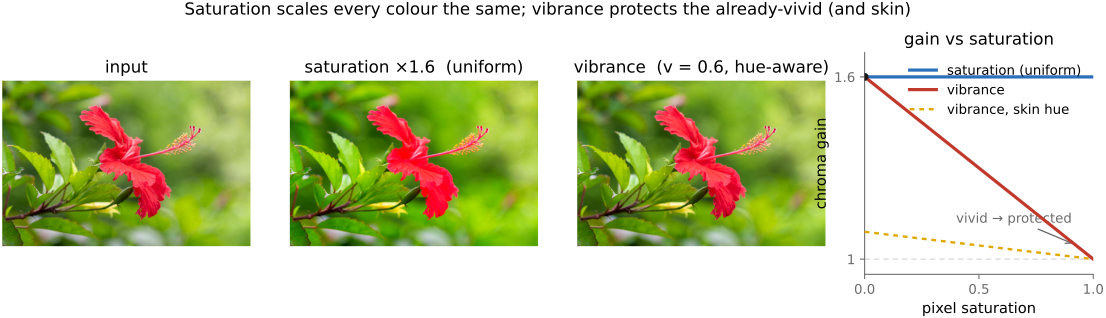
Vibrance is a gentler cousin: it boosts the saturation of muted colors more than already-vivid ones, and typically spares skin tones, so portraits do not turn garish (Figure 4.4.12). It is the same formula, but with the constant $s$ replaced by a per-pixel gain that is large where a pixel is dull and fades to nothing where it is already colorful (and near skin hues):
Here $\text{sat}$ is the pixel's current saturation — for instance the hue-saturation-value (HSV) quantity $S = (\max - \min)/\max$, or the chroma magnitude divided by luminance — $v$ is the vibrance amount, and $w_\text{skin}(\text{hue})$ is a hue weight near $0$ on skin and orange tones and $1$ elsewhere (set it to $1$ everywhere for a skin-agnostic version). Because the gain carries the $(1 - \text{sat})$ factor, a flat gray-blue sky gets the full boost while an already-vivid flower, or a face, barely moves. Photographers reach for a touch of vibrance as a finishing move — cameras tend to render colors a little flat — but it is easy to overdo (Figure 4.4.11).
Since these edits (and the editor's sliders) speak HSV, it is worth writing the conversion down. With $M=\max(R,G,B)$, $m=\min(R,G,B)$, and chroma $C=M-m$:
$$ V = M, \qquad S = \begin{cases} C/M & M>0\\ 0 & M=0\end{cases}, \qquad H = 60^\circ \times \begin{cases} \big((G-B)/C\big) \bmod 6 & M=R\\ (B-R)/C + 2 & M=G\\ (R-G)/C + 4 & M=B.\end{cases} $$
Value is just the brightest channel, saturation the chroma as a fraction of that value, and hue the angle around the color wheel — a cheap polar view of color that the vibrance gain above (and hue-selective grades) read off directly. The closely-related HSL swaps value for lightness $L=(M+m)/2$. Both are computed on the same gamma-encoded values as the saturation edit, so their "value"/"lightness" is not a true luminance — a convenient control coordinate, not a photometric one.
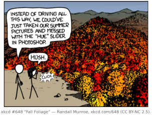
Figure 4.4.11. xkcd #648 "Fall Foliage" — Randall Munroe, xkcd.com/648 (CC BY-NC 2.5).Figure 4.4.12.Saturation versus vibrance. Left, the input — a vivid red flower against muted green foliage. Center, a uniform saturation boost (constant $s = 1.6$): the dull foliage improves, but the already-vivid flower is pushed past the gamut and clips, its petals turning flat and garish, because every pixel is scaled the same amount. Right, vibrance (per-pixel gain $g$, here $v = 0.6$ so the gray-point gain $1+v$ matches $s$): the muted foliage gets the full boost while the saturated flower barely moves, because the gain fades as a pixel's own saturation rises. The fourth panel plots the chroma gain each method applies against a pixel's saturation — flat at $s$ for saturation, tapering from $1+v$ down to $1$ for vibrance, and damped further on skin hues (dashed). Same intended "more color," very different treatment of the colors that were already fine.
One caveat: "how far from gray" and "leave lightness alone" both depend on the color space you measure them in, and doing this well means scaling chrominance in a perceptually uniform space rather than naively in RGB. That choice of space — and why skin needs protecting at all — is genuinely the subject of the color part, so it is what we defer to Color technology; the mechanics are the two equations above. Both saturation and vibrance are color operations, not tone operations.
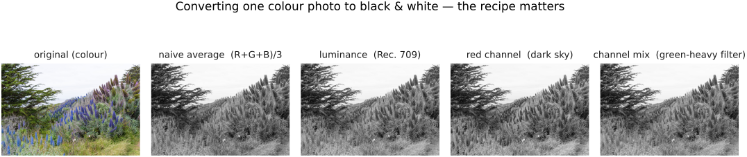
"Convert to black and white" sounds like a single operation, but it is the cleanest everyday illustration of the non-orthogonal, non-negative theme (from the color chapters of the previous part) turned into a question of intent. You are projecting three numbers to one — an inherently many-to-one, lossy map — so there is no single correct gray; there are many valid answers, and the right one depends on what you want, not on correctness (Figure 4.4.13). The general recipe is a weighted sum
$$ \text{grey} = w_R R + w_G G + w_B B, \qquad \sum_i w_i = 1, $$
with the constraint chosen to hold exposure, and the interesting questions are which weights and in which space.
Figure 4.4.13.One color photo, many grays. The same image converted by: a single channel (R, G, or B); a flat average $(R{+}G{+}B)/3$; weighted luminance (Rec. 601/709); a red-filter channel mix that darkens a blue sky for dramatic clouds; and an isoluminant pair — a red and a green of equal luminance — that collapses to the same gray, erasing the edge between them. The conversions genuinely differ, proving there is no one right answer.
The options form a ladder of sophistication. Pick a single channel (R, G, or B): fast, occasionally useful — the green channel is close to luminance and usually least noisy, the red channel smooths skin and darkens skies — but it throws away two-thirds of the data. Average $(R+G+B)/3$ is simplest but perceptually wrong: it makes blue as bright as green, so skies and foliage come out muddy. Weighted luminance is the perceptual default — the cone-weighted sum where green dominates and blue counts little, the Rec. 601 ($0.299/0.587/0.114$) or Rec. 709 ($0.2126/0.7152/0.0722$) weights from earlier — but in which space? The recurring luma-versus-luminance distinction bites here: the cheap version weights the gamma-encoded values (luma $Y'$, what most software does), the radiometrically correct version weights linear RGB (luminance $Y$) and re-encodes, and the two give visibly different grays (linear-light is darker in saturated reds and blues). One can also take lightness, not luminance — the perceptually uniform L\* from CIELAB — or the UI shortcuts HSL "lightness" $(\max + \min)/2$ and HSV "value" $\max(R, G, B)$, each a different gray again.
The expressive end of the ladder is the custom channel mixer: choose the weights yourself (keeping $\sum w_i \approx 1$ to hold exposure). This is Lightroom and Photoshop's black-and-white mixer, and it is the digital descendant of putting a color filter on black-and-white film — a red filter darkens a blue sky for dramatic clouds (Ansel Adams's black skies are a red filter on panchromatic film), a yellow or green filter lightens foliage, an orange filter smooths skin. So a conversion is really a decision about how each color should map to gray. The hard case exposes the lossiness directly: two distinct hues with the same luminance (a red and a green of equal brightness) map to the same gray, erasing the edge between them. Contrast-preserving decolorization methods (Color2Gray, Gooch et al. 2005; Grundland & Dodgson 2007) optimize the mapping to keep color contrast rather than only luminance — the principled answer to "the green apple and the red apple should not vanish into one gray."
Video 4.4.1. Video: Color2Gray: Salience-Preserving Color Removal — Amy A. Gooch, Sven C. Olsen, Jack Tumblin, Bruce Gooch 2005 (YouTube).
💡 Big lesson callback — black-and-white is a lossy projection
Converting to gray is a $3 \to 1$ projection: many-to-one, non-invertible, and therefore underdetermined. There is no single correct gray — only choices that trade perceptual fidelity against drama against contrast preservation. This is the same non-orthogonal, non-negative lesson from Human Vision, now staring back at you from a routine menu command.
Once a point operation is any fixed curve f, there is a cheap trick that applies to all of them at once. If pixel values come from a small finite set — the 256 levels of an 8-bit channel, say — there is no need to evaluate f at every pixel. Evaluate it once per possible value, store the 256 answers in a small table, and then for each pixel just look up its result. This precomputed table is a look-up table (LUT), and it turns an arbitrarily complicated tone curve into a single array index per pixel — the same cost whether f is a gamma curve, an S-curve, or a hand-drawn spline.
A 1-D LUT is exactly this: three independent per-channel curves, into which exposure, contrast, levels, and gamma all collapse. It cannot express a cross-channel effect, because each output channel depends only on its own input channel. A 3-D LUT lifts that limit: it maps a whole (R, G, B) triple at once, so it can do the things a per-channel curve cannot — white balance, saturation, a full color grade. The price is size: a dense 3-D table would be enormous, so it is sampled on a coarse grid (the .cube files of video carry a few dozen entries per axis) and interpolated between samples. LUTs are everywhere once you look: the gamma encode/decode step is a 1-D LUT, a creative "film look" ships as a 3-D LUT, and the same trick doubles as a speed optimization — precompute any expensive per-value function once, then index it (the basis of fast fixed-point and 8-bit pipelines).
Tone and color tools developed separately for stills and for motion pictures, and the two vocabularies never fully merged. Color grading is the motion-picture craft, and it is worth meeting on its own terms because it is a separate discipline from the stills/radiometric editing the rest of this chapter describes: less concerned with physical radiance, far more concerned with the look of a film, and equipped with its own tools and idioms.
The colorist's primary controls are the lift / gamma / gain wheels. Rather than a single exposure or contrast slider, these split the tonal range into three overlapping bands — lift for the shadows, gamma for the midtones, gain for the highlights — and each wheel carries a color offset as well as a level, so you can, say, cool the shadows and warm the highlights independently. Corrections come in two layers: primary corrections act on the whole frame (overall balance and exposure), while secondary corrections are qualified — restricted to a range of hue or luma, or to a tracked mask — so you can grade just the sky, or one actor's shirt, without touching the rest.
The pipeline underneath is built for range and consistency. Footage is usually captured in a camera log encoding — Sony's S-Log, or Log-C from ARRI (the cine-camera maker) — which packs a wide dynamic range into the file the way log encoding always does (a multiplicative range becomes an additive one, the recurring lesson). Grading then happens inside a color-management framework, most prominently the Academy Color Encoding System (ACES), which defines common working and interchange spaces so that material from different cameras grades and intercuts predictably. The finished look is then frozen and shipped as a 3-D LUT — the .cube files from the lookup-tables section above — applied per frame, which is precisely why 3-D LUTs matter here: they are the delivery format for a grade.
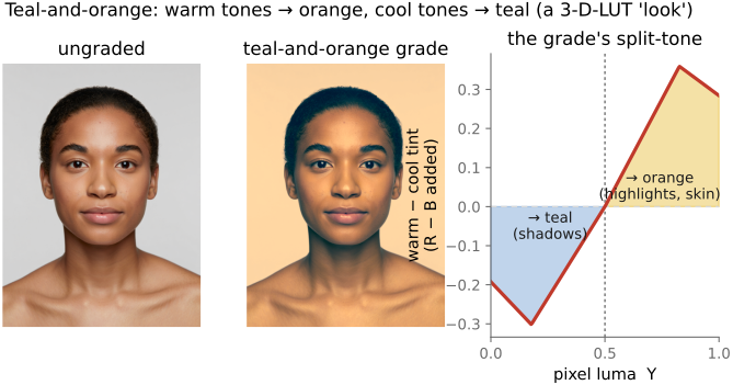
A common example is the teal-and-orange look. Skin tones are pushed toward warm orange; everything else is pulled toward the complementary teal. Because orange and teal sit opposite each other on the color wheel, the result is a built-in complementary contrast that makes people pop off the background (Figure 4.4.14). The look was popularized by the digital grade of O Brother, Where Art Thou? (2000) — among the first features finished entirely as a digital intermediate (the Coen brothers, cinematographer Roger Deakins) — and it has been imitated to the point of cliché ever since.
Figure 4.4.14.The teal-and-orange grade on a real frame. Left, the ungraded photo — warm skin against cool water and sky. Center, the grade applied: the warm, sun-lit tones (skin especially) are pushed toward orange while the cooler shadows and the water shift toward complementary teal, so the subject pops off the background by built-in color contrast. Right, the mechanism as a split-tone — the warm-minus-cool tint the grade adds as a function of a pixel's luma: teal below the mid-gray split point, orange above it. This is a fixed $\text{RGB} \to \text{RGB}$ mapping, the kind of creative look a colorist freezes and ships as a 3-D LUT (.cube) applied per frame.
The stills world has a close cousin: Lightroom's hue-saturation-lightness (HSL) / color-mixer and color-grading panels do much the same hue-selective work a colorist does with secondaries. We mostly speak the stills/radiometric dialect in this book, but the operations underneath are the same point operations seen through a different craft. The grading toolkit ties back to #Lookup tables (3-D LUTs as the delivery format), to Color technology (color management, log encoding, ACES), and forward to tone mapping (the dynamic-range side of the same problem).
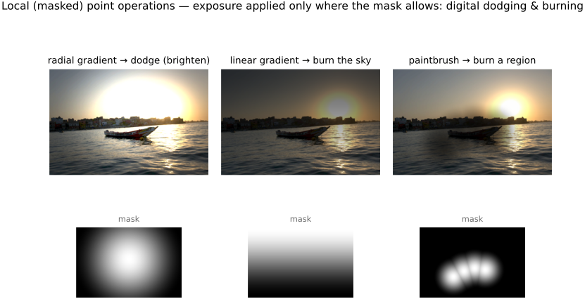
One loose end. We defined a point operation as depending only on a pixel's value, the same rule everywhere — yet editors constantly let you apply these very tools locally, through a selection or a mask: brighten only the sky, add contrast only to the face. Strictly, that is no longer a point operation, because the result now depends on where the pixel is and not just its value — it is the digital descendant of the darkroom's dodging and burning. Selections come in many flavors — by value or color (the magic wand), by a painted brush, by a gradient ramp (linear or radial), edge-aware (snapping to object boundaries), and increasingly by AI semantic segmentation (segment-anything-style). The edge-aware kind hints at a theme we will keep meeting: an edge-preserving selection treats two pixels as belonging together when their colors are similar — an affinity — which is the very idea that drives the bilateral filter. We flag selections here so the boundary of "point operation" is clear; the machinery is the bridge to local tone mapping and the edge-preserving filtering of later chapters.
The connection to the darkroom is exact (Figure 4.4.15). Wherever the mask is bright, the adjustment acts; where it is dark, the pixel is untouched. Run a local exposure through a mask and you have reinvented dodging (locally brightening — holding light back in the printing easel) and burning (locally darkening — giving extra exposure): the only difference is that the mask is now a soft digital matte instead of a piece of cardboard waved over the paper. A radial gradient lifts a face out of the shadows; a linear gradient is the graduated-ND filter that holds back a bright sky; a painted brush burns down one distracting highlight. Everything earlier in the chapter — exposure, contrast, the tone curve — becomes a local tool the moment it is gated by a mask.
Figure 4.4.15.Local (masked) point operations — digital dodging and burning. The same point operation (here exposure) is applied only where a mask allows. Radial gradient: dodge (brighten) the center, lifting the subject. Linear gradient: burn the top, the digital graduated-ND that tames a bright sky. Paintbrush: burn a chosen region. The lower row shows each mask (white = full effect). Interactive: pick the mask shape and the adjustment (exposure for dodge/burn, or contrast), set the amount, and drag the mask's handle — or, in brush mode, paint directly on the image.
Recap: big lessons of this chapter
(L2.19) — additive vs. multiplicative → choice of encoding
The single most useful question to ask of any tonal operation is whether it is fundamentally additive or multiplicative, because the answer dictates the right encoding. A multiplicative change — scaling the light, the way exposure does — is natural in linear light (and becomes a plain addition in log). An additive change in display space — brightness, a fixed offset — lifts every value by the same amount, regardless of how much light there was to begin with. Light itself is multiplicative (double the photons, double the radiance), and perception is closer to multiplicative too: contrast is about ratios, not differences — the step from 1 to 2 looks like the step from 100 to 200. That is why so much of imaging prefers linear or log over a naive offset. Keep asking "additive or multiplicative?" and the choice of space usually answers itself.
(L4.2) — exposure scales linear light (a multiply) or shifts log values (an add)
Changing exposure is a multiplication of linearly-encoded values ($L_\text{out}=k\,L_\text{in}$, with $k=2^{s}$ for $s$ stops) — equivalently an addition in log/stops ($\log L \mapsto \log L + \log k$). In gamma-encoded data it is neither, so the right move is to convert to linear (or log), apply, convert back. If you must work in place, the exact gamma-space map is still a multiply, but by $k^{1/\gamma}$ rather than $k$: $L_\text{out}=k^{1/\gamma}\,L_\text{in}$ — the kind of off-by-a-gamma error that bites silently. This is the cleanest case of L23, "do the physics in linear light, apply gamma last."
(L4.3) — contrast is a pivot: choose what stays put
A contrast change rotates values about a chosen pivot: $L_\text{out} = p + g\,(L_\text{in}-p)$. The pivot $p$ is exactly what is left unchanged, and it also decides whether the picture gets brighter or darker overall — a high pivot pulls most of the image down (darkening), a low pivot pushes it up (brightening). Unlike exposure, contrast is not radiometrically meaningful — it is a stylistic stretch — so the encoding matters less (no single space is "correct"); what matters is a sensible pivot, and the sensible pivot does depend on the space: roughly 18% mid-gray in linear light, the numeric midpoint in gamma or log. Pick the pivot deliberately — it is the whole character of the operation.
callback — black-and-white is a lossy projection
Converting to gray is a $3 \to 1$ projection: many-to-one, non-invertible, and therefore underdetermined. There is no single correct gray — only choices that trade perceptual fidelity against drama against contrast preservation. This is the same non-orthogonal, non-negative lesson from Human Vision, now staring back at you from a routine menu command.