4.8 Neighborhood operations and convolution⧉
PS2 implements box/Gaussian blur, gradients, sharpening, and the bilateral filter. → Problem sets (appendix).
Blur is not something that happens to a pixel; it happens between pixels. A point of light is never recorded as a single lit pixel: diffraction and the imperfections of real glass spread it into a small blob a few pixels wide, and every recorded value is a mixture of the light meant for that spot and the light that leaked in from its neighbors. That is the linear-operator view, one matrix $A$ applied uniformly across the frame (Imaging as a linear system).
In the previous chapter every operation was a point operation — the output pixel depended only on the input pixel sitting at the same location, run through a single curve. Here we let the output pixel consult its neighborhood, a small window of surrounding pixels, and combine them. This is the third of the three operation families we laid out (range, domain, neighborhood); we are now firmly in the neighborhood column. Blurring, sharpening, edge detection, and most of the noise-cleaning filters of later chapters all live here, and nearly all of them rest on a single operation called convolution.
4.8.1 Motivation: blur and sharpen⧉
Two everyday edits motivate the machinery, and they pull in opposite directions.
The first is blur. You blur on purpose constantly — to soften skin in a portrait, to fake a shallow depth of field, to knock down noise, or as an internal step in a larger algorithm (downsampling, building the pyramids of a later chapter, extracting the base layer of a local tone map). But blur also shows up uninvited, baked in by the optics: diffraction at the aperture, spherical aberration and other lens flaws, defocus, camera shake, and subject motion all smear a point of scene light into a blob on the sensor. Each sensor pixel therefore stores a weighted average of light from a small patch of the scene — exactly the picture from the lecture, where a pixel's value is the local average of the colors in front of it. Understanding that averaging precisely is what later lets us hope to undo it.
The second is sharpen — making an image crisp, undoing blur or at least faking its opposite. Sharpening is the mirror instinct: instead of mixing a pixel with its neighbors, accentuate how it differs from them. It turns out to be built from exactly the convolution machinery below — so we set it up here but give it its own chapter, Sharpening, immediately after.
Both deserve precision for the same reason. Once we know exactly how blur mixes neighbors, we can pose the harder question of how to remove it. That removal — deconvolution or deblurring — gets a whole later chapter, and it is tractable only because blur is a linear operation we can write down and, with care, attempt to invert. The payoff for being careful here is large, so let us be careful.
4.8.2 Convolution 101⧉
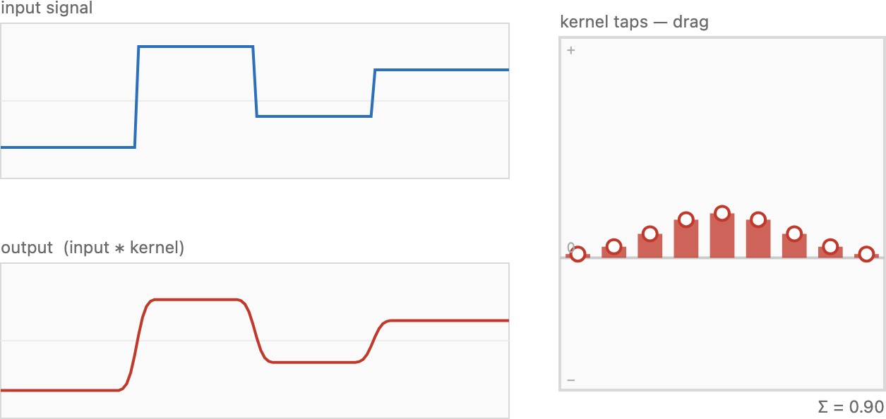
Start with blur, the easy direction. The recipe is almost embarrassingly simple: replace each pixel by a weighted average of its neighbors. For a gentle blur, give a pixel mostly to itself with a little spilled in from its immediate neighbors; for a heavy blur, spread the weight across a wider window. The little table of weights that says how much each neighbor contributes is the convolution kernel (written g, sometimes k). The kernel defines the operation: pick the weights and you have picked the blur.
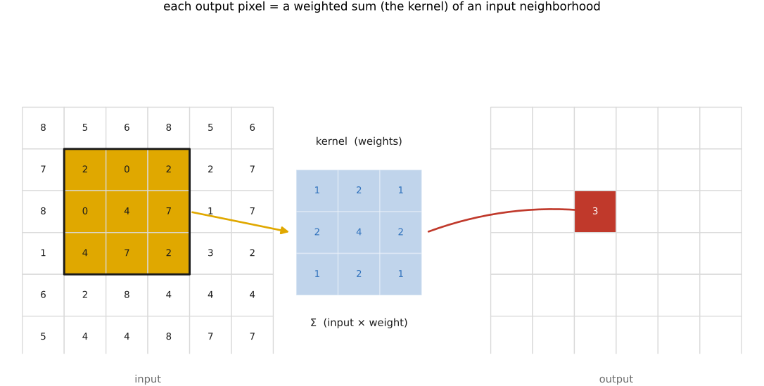
Two properties of this scheme are worth naming, because together they pin down the family of filters we can handle cleanly. First, it is linear: each output pixel is a weighted sum of input values with fixed weights, so scaling the input scales the output, and adding two images adds their outputs. (Formally, an operation $F$ is linear when $F(a\,I + b\,J) = a\,F(I) + b\,F(J)$ for any images $I, J$ and scalars $a, b$.) Second, it is shift-invariant: the same kernel applies at every pixel, so the operation does not care where in the image you are. Shift the input and the output just shifts to match. An operation that is both is a linear shift-invariant (LSI) filter, and convolution is precisely the LSI operation — no more, no less.
Both conditions are real constraints, and it helps to watch one break. A graduated neutral-density filter — the kind that darkens the sky at the top of the frame while leaving the foreground alone — multiplies each pixel by a factor that depends on its row, say $(1 - y/y_\max)$. That is still linear (scaling the input scales the output), but it is emphatically not shift-invariant: slide the image down and the darkening falls on different content. So it is a linear operation that is not a convolution. Convolution is the well-behaved special case where the rule is identical everywhere, and that uniformity is exactly what later lets the Fourier transform pry it open.
A convolution replaces each pixel by a weighted combination of its neighbors — in practice usually a local one (a small window). Two things define it: the weights depend only on the relative position of each neighbor (not on where you are or what the values are), and they are the same everywhere in the image. That sameness is shift-invariance: slide the input and the output just slides to match. "Linear + shift-invariant + local" is the whole definition, and it is why a convolution is captured by one small kernel, why blur, gradients, and sharpening are all "one stencil applied everywhere," and why the next chapter's Fourier transform can diagonalize it.
Convolution assumes one kernel applied everywhere (shift-invariant). Much real optical blur breaks that. Defocus blurs each object by an amount set by its depth, so a scene with near and far subjects holds many blur sizes at once. Camera shake is mostly a rotation of the camera, which smears the corners more than the center and along curved paths — one motion, but a different streak at every pixel. Spherical aberration, coma, and field curvature worsen toward the frame edge, and chromatic aberration even differs per color channel. None of these is "a single kernel convolved over the whole image" — each breaks the shift-invariance that lets the linear operator collapse to a convolution (Imaging as a linear system). The saving grace is locality: zoom into a small enough patch and the blur is approximately constant there, so it behaves as a local convolution — the image is a patchwork of slowly-varying kernels (a spatially-varying PSF). That is why the clean intuitions built in this chapter — blur is linear, deblurring is inverting a linear system, and how recoverable it is depends on which frequencies the kernel destroyed — still largely hold; what changes is bookkeeping (a field of kernels, or a physical motion model), not the core lesson. The full, global treatment of camera-shake blur is in Blind deblurring.
Why insist on linearity at all? Because linear operations are the ones we have tools for. If blur is linear, then deblurring is inverting a linear system, and linear algebra can tell us in advance how hard that will be — whether the blur discarded information for good or merely scrambled it recoverably (the deblurring chapter's spoiler: usually somewhere in between). A nonlinear smear offers no such handle. One caveat to flag now and revisit: because blur is a physical, linear mixing of light, it acts on linear-light values, not on the gamma-encoded numbers a PNG stores. Blurring the gamma values is a common, visible mistake; we return to it in the blur zoo.
The algorithm itself is a short loop. Zero the output, then for every output pixel, walk over the kernel, multiply each input neighbor by its weight, and accumulate:
for each output pixel (x, y):
    out[x, y] = 0
    for each kernel offset (x', y'):
        out[x, y] += in[x + x', y + y'] · g[x', y']
assuming the kernel's coordinates are centered on zero. Read it back in words: each output pixel is the sum, over its neighborhood, of input value times the weight sitting on it. That is the entire computation — and yet a subtle sign issue lurks inside it, which is the subject of the next section.
4.8.3 The flip: where-from vs. where-to⧉
The loop just written reads in[x + x'] — the neighbor ahead by the offset. The textbook definition of convolution reads the neighbor behind; it subtracts the offset:
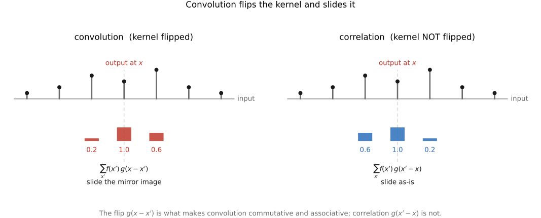
In words: to get the output at $x$, sum over all input positions $x'$, each weighted by the kernel evaluated at $x - x'$ — the kernel is flipped (and slid) before it is multiplied in. Why the flip, and does it matter?
The flip is the difference between where light goes to and where light comes from. The physical, forward model says light at scene position $x$ lands, blurred, at sensor positions $x + x'$ for the offsets in the kernel; light spreads outward. But when we compute the output at a fixed pixel $x$, we are asking the backward question: which input pixels contributed here? The answer is the ones at $x - x'$. The minus sign is nothing but the bookkeeping of inverting "where-to" into "where-from."
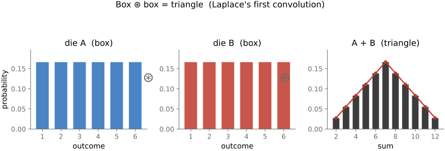
Convolution was first written down by Laplace, studying the sum of two random variables. If $X$ and $Y$ are independent with known distributions, the distribution of $X + Y$ is their convolution — and the flip falls out for free. To ask "how likely is $X + Y = x$?", enumerate the ways it can happen: $X = x'$ paired with $Y = x - x'$, for every $x'$. The second variable is forced to be the sum minus the first, and you add up the products of probabilities over all $x'$. That $x - x'$ is exactly the convolution flip — here not a convention but a logical necessity. The cleanest instance is two dice: each die is a flat distribution over 1–6 (a one-dimensional box), and the distribution of the total is that box convolved with itself, a triangle peaking at 7 (Figure 4.8.4). This is why, throwing two dice, a sum of 7 is much more likely than a 12: there are six ways to roll a 7 (1+6, 2+5, 3+4, 4+3, 5+2, 6+1) but only one way to roll a 12 (6+6), so a 7 comes up six times as often — the middling totals win because there are simply more ways to reach them. A box convolved with a box is a triangle; the box returns in the blur zoo.
Does the flip ever bite in practice? Only for asymmetric kernels. A box and a Gaussian are symmetric — flipping them changes nothing — so for the blurs that dominate this chapter you can ignore the flip entirely and the loop above is correct. But a derivative kernel like [−1, +1] is antisymmetric, and there the flip reverses the sign of the result, so it genuinely matters for gradients and sharpening. Drop the flip and you get a closely related operation called correlation, differing only in that flip. Correlation is perfectly useful — it is the natural operation for template matching, "where in the image does this patch appear?" — but it lacks convolution's clean algebra (the symmetries below), which is why convolution is the one we build the theory on.
4.8.4 Properties: the impulse, normalization, symmetry, commutativity⧉
A handful of properties make convolution pleasant to work with, and the slickest way to expose them is to feed the filter the simplest possible input: one bright pixel on a black background, the impulse $\delta$ (the discrete Dirac / Kronecker delta — one at the origin, zero everywhere else).
Convolve an impulse with a kernel and you get the kernel back, stamped at the impulse's location. The flip explains why: every output pixel asks "where did my light come from?", and the only nonzero input is the single bright pixel, so each output simply picks up the kernel weight that connects it to that pixel — tracing out the kernel. This output carries a name borrowed from optics: the point spread function (PSF), or impulse response. It is literally how the system spreads a single point of light — the very blob you saw around the streetlight. So the kernel, the impulse response, and the PSF are three names for one thing, with an immediate practical corollary: to discover what a filter does, feed it an impulse and read off the kernel. This is the single best debugging input for convolution code, and we will lean on it.
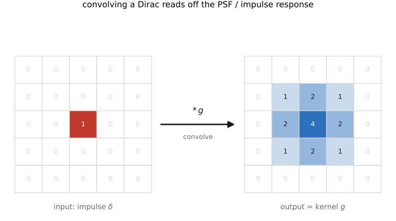
The impulse trick is also the fastest way to debug filtering code, so keep a few hand-checkable inputs at the ready. Convolve an impulse and the output is your kernel, laid out and flipped — read it off weight by weight to catch a wrong number, an off-by-one in the centering, and the flip (convolution vs. correlation) at a glance. A constant image must come back unchanged — and it does exactly when the weights sum to one, so a constant test verifies normalization. An off-center single-1 shift kernel translates the whole image by exactly that offset, which checks the sign and direction of your indexing (and exposes a stray flip immediately). A half-plane — black on one side, white on the other — shows the border behavior and the edge response. Do the very first test in 1-D (a 1×3 kernel), where every output pixel is computable by hand, before trusting anything in 2-D. (See the impulse picture in Figure 4.)
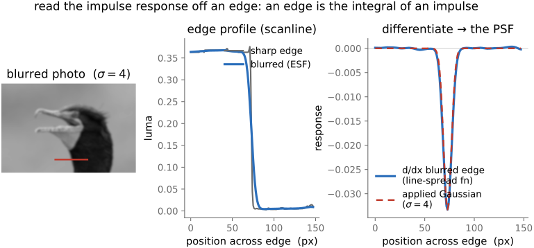
A clean impulse is a luxury you rarely have in a real photo, but a sharp edge does just as well, because a step is the running sum of an impulse. So the way a blur smears an edge is the integral of the impulse response along the edge normal: sample a scanline across a sharp boundary (its profile is the edge-spread function), differentiate it, and the bump you recover is the PSF's 1-D projection. Feed a blurred photo a real edge and the derivative hands back the very kernel that blurred it (Figure 4.8.6) — the impulse test run on an edge instead of a lone pixel, and the everyday way lens sharpness (the modulation transfer function (MTF) of the next chapter) is actually measured.
The identity element follows at once: convolving with the impulse leaves the image untouched, $I * \delta = I$, because reading "where-from" with a kernel that points only at yourself just copies you. The remaining properties:
- Normalization. For a blur to preserve the image's overall brightness — neither darkening nor brightening it — the kernel weights must sum to one. A blur whose weights summed to 0.9 would dim the picture by 10% everywhere. (The rule of thumb is "normalize your kernels," but not always: a gradient kernel sums to zero on purpose, because it measures change, not brightness.) In practice the easy move is to build a kernel and then divide by its sum.
- Commutativity and associativity. $I * g = g * I$, and $(I * g) * h = I * (g * h)$. The first says it does not matter which operand you flip — the same logic as the dice, where all that matters is that the two offsets sum to the target. The second says a chain of filters can be pre-combined into one: blur-then-sharpen is a single convolution with $g * h$, computed once. These symmetries are exactly what the flip buys you; correlation has neither.
- Linearity, already noted, is the deepest property — it is the reason the next chapter's Fourier transform can diagonalize convolution into a simple per-frequency multiplication, and the reason deblurring is even thinkable.
4.8.5 Nitty-gritty: finite images⧉
Two practical wrinkles before the kernels themselves.
First, the kernel must be centered. Our images place $(0, 0)$ at the top-left corner, but a blur kernel is naturally centered on the pixel it is computing — its weights run from $-r$ to $+r$ around the middle, where $r$ is the kernel radius, so the full size is $(2r+1) \times (2r+1)$. An off-by-one here shifts the whole image by a pixel; an impulse test catches it instantly, because the blob lands off-center.
Second, our images are not infinite. When the kernel hangs off the edge of the image it asks for pixels that do not exist, and we must decide what they mean — the same edge-handling choice we set up with the safe accessor in Image representation. The usual options: zero / black padding (treat the outside as black — but this darkens the borders, since a blur there averages in fake black), clamp / edge padding (repeat the nearest edge pixel — simple and safe), and mirror / reflect padding (fold the image back on itself — usually the best default, avoiding both the darkening of zero-padding and the streaking of clamp). Pick one deliberately; the figure library's gaussian_blur uses reflect.
4.8.6 A blur zoo⧉
With the mechanics settled, the only choice left is the kernel's shape. Two are worth knowing.
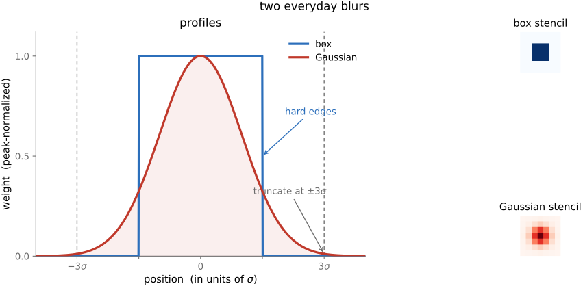
The box filter is the crudest: every pixel in a $(2r+1) \times (2r+1)$ window gets equal weight, $1/(2r+1)^2$, so the weights sum to one. It is a plain average of the neighborhood. It blurs, it is cheap, and it has a flaw — its hard square edge makes it directional (it blurs more along the diagonals) and it produces faint ringing the Fourier chapter will explain. Use a box filter when speed matters more than quality.
The Gaussian is the workhorse. Its weights fall off smoothly with distance from the center, following the bell curve
where $r$ is the distance to the center and $\sigma$ (the standard deviation) sets the width — the blur's "radius" in spirit. Read it back: a neighbor's weight decays exponentially with the square of its distance, so nearby pixels count for a lot and far ones fade smoothly to nothing. The Gaussian is smooth, rotationally symmetric (no directional bias), and — as the next chapter shows — uniquely well-behaved in frequency, which is why it is the default blur almost everywhere.
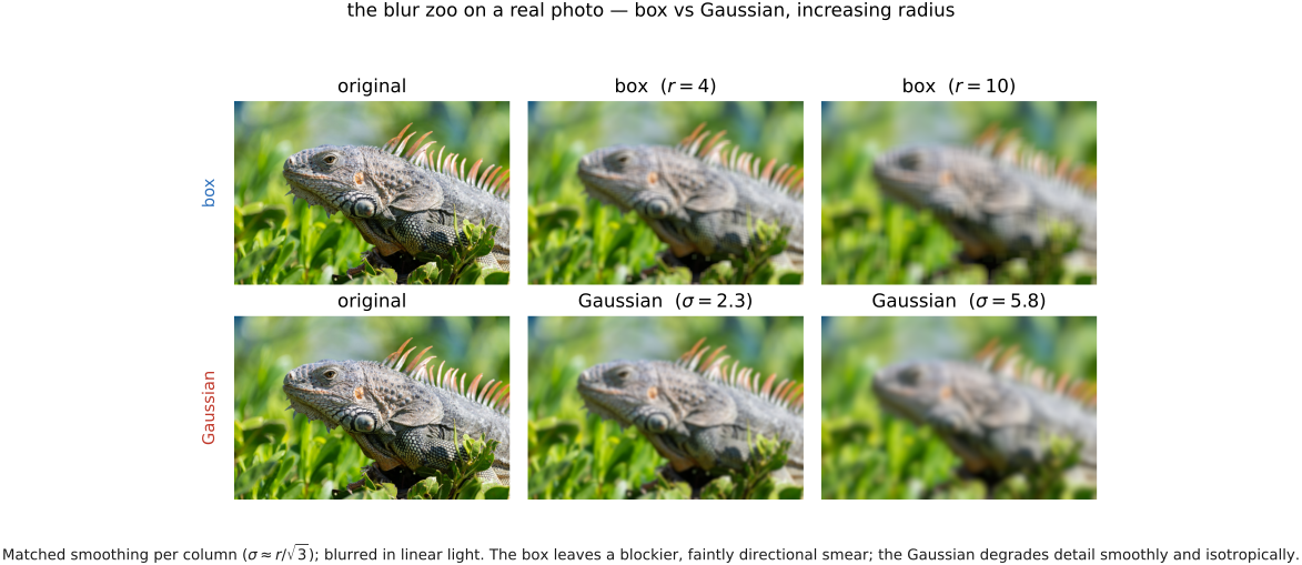
Run both on an actual photograph and the difference in feel is plain: the box smears fine texture into faintly blocky, slightly directional mush, while the Gaussian dissolves it smoothly and isotropically. Use a Gaussian when the blur should look natural (Figure 4.8.8).
One technicality: the Gaussian never actually reaches zero — it has infinite support, positive everywhere. We cannot use an infinitely large kernel, so we truncate it, treating it as zero beyond some radius. A radius of 3σ is the standard choice: by three standard deviations the weights are negligible (well under 1% of the peak), so cutting them costs nothing visible while keeping the kernel finite. After truncating, renormalize so the surviving weights still sum to one.
Now the encoding warning comes due. Because blur is the physical mixing of light, a Gaussian blur should be computed in linear light — decode the gamma-encoded image to linear, blur, then re-encode. Blur the gamma values directly and the result is subtly wrong, most visibly where a bright and a dark region meet: the blurred transition bows toward dark, because gamma encoding is nonlinear and the average of two encoded values is not the encoding of their average. For gentle blurs on ordinary images you may not notice; for strong blurs, bright highlights, or anything you plan to deconvolve, it matters. (imageops.gaussian_blur operates on the array it is handed; the figure scripts feed it linear-light values whenever the physics demands it.)
4.8.7 Separability⧉
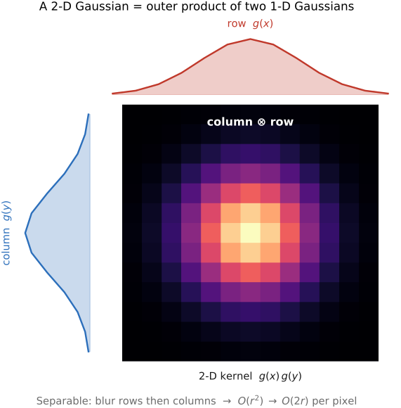
A $(2r+1) \times (2r+1)$ Gaussian appears to cost $(2r+1)^2$ multiplies per output pixel — quadratic in the radius, which is painful for a big blur. There is a beautiful escape. A 2-D filter is separable if it can be written as one 1-D filter applied along the rows followed by another along the columns — formally, the 2-D kernel is the outer product of two 1-D kernels. The Gaussian is separable, because $\exp(-(x^2 + y^2)/2\sigma^2) = \exp(-x^2/2\sigma^2) \cdot \exp(-y^2/2\sigma^2)$: a 2-D Gaussian is a horizontal 1-D Gaussian times a vertical one. (So is the box, trivially.)
The payoff is a cost win, not just elegance. Instead of one $(2r+1)^2$ pass you do two $(2r+1)$ passes — blur every row with a 1-D Gaussian, then blur every column. The cost per pixel drops from $O(r^2)$ to $O(2r)$, linear in the radius. For a $\sigma = 10$ Gaussian (radius 30, a 61×61 kernel) that is the difference between ~3700 multiplies per pixel and ~120 — a 30× speedup, and the reason large Gaussian blurs are practical at all. Separability is the first of several "do it in 1-D twice" tricks that recur through the book.
4.8.8 Gradient and oriented filters⧉
Not every useful kernel blurs. The most important non-blurring kernel measures change — how fast the image brightens or darkens as you step across it — and that turns out to be the foundation of edge detection.
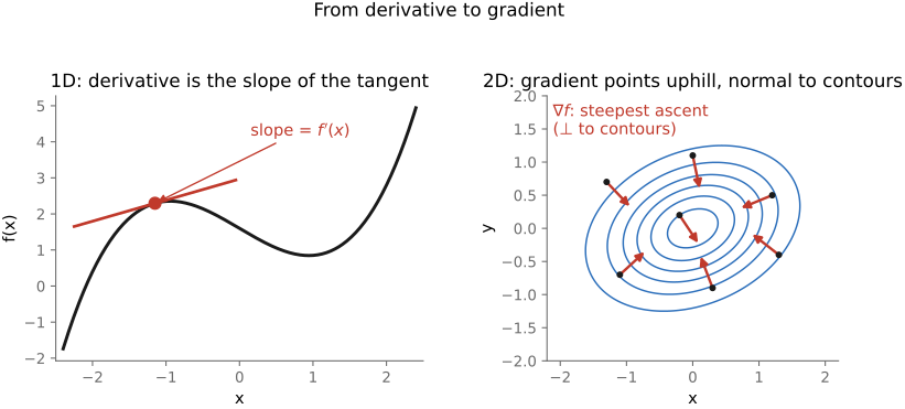
Recall from calculus that a derivative is a difference over a distance — the slope of the tangent (Figure 4.8.10, left). For a discrete image the simplest finite-difference kernel is [−1, +1], which subtracts a pixel from its right neighbor to estimate the horizontal derivative $I_x = \partial I / \partial x$. (Note the weights sum to zero — this kernel measures change, not brightness, so it is not normalized to one; and it is antisymmetric, so the flip genuinely matters.) The transpose, [−1; +1] stacked vertically, estimates the vertical derivative $I_y$. Where the image is flat the difference is zero; where it crosses an edge the difference spikes. So a derivative kernel lights up edges and ignores smooth regions.
A grayscale image is a two-dimensional function — a brightness landscape with hills and valleys — so its derivative is not a single number but a gradient: a vector that, like the slope of a hill, points in the direction of steepest brightening and is perpendicular to the contours of constant brightness (Figure 4.8.10, right). Its two components are exactly the horizontal and vertical partials, $I_x$ and $I_y$, which is why we estimate each with its own finite-difference kernel.
Taking an image derivative is a convolution. With finite differences it is the obvious little stencil — [−1, 0, +1], or Sobel — and with the proper mathematical treatment a continuous derivative is convolution with the derivative of a smoothing kernel (the derivative-of-Gaussian). So gradients, edges, the Laplacian, and unsharp masking are all linear shift-invariant filters (L4.5) — which is exactly why they have clean Fourier behavior, why edge detection is "just" filtering, and why combining a derivative with a blur (Sobel, derivative-of-Gaussian) is the natural noise-robust way to measure change.
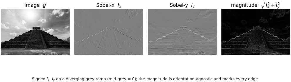
Raw finite differences are jumpy — they amplify noise, since noise is exactly small high-frequency wiggle. The standard fix is the Sobel kernel, which pairs a derivative along one axis with a little smoothing along the other:
a horizontal difference (the −1, 0, +1 across each row) blurred vertically (the 1, 2, 1 weighting down the columns) for noise robustness. Its transpose gives the vertical Sobel.
Stacking the two partials into a vector gives the image gradient $\nabla I = (I_x, I_y)$, the brightness-landscape gradient of Figure 4.8.10 applied to a real image. Two numbers fall out of it, both central to vision:
The magnitude is large exactly at edges and near zero in flat regions — a raw edge-strength map — and the orientation says which way the edge runs. Threshold the magnitude and you have a crude edge detector; the careful version (non-maximum suppression, hysteresis — the Canny detector) is a forward reference to the features chapter, but the gradient computed by two Sobel convolutions is its beating heart.
Blur, gradients, and their kin all share the same comfortable assumption: one kernel, applied the same way everywhere. Before we lean on it, it is worth asking how well that assumption actually holds for the blur a real camera produces — because that is where the clean theory meets messy optics. (Sharpening, the inverse instinct that undoes a blur, is its own chapter, Sharpening, right after this one; deconvolution — undoing blur exactly — comes later still.)
4.8.9 Is imaging blur usually a shift-invariant convolution?⧉
This whole chapter has modeled blur as a convolution — one kernel, applied identically everywhere. It is worth asking how often that is actually true of real camera blur, because the true answer is usually not, and knowing where the model breaks tells you when the clean linear-shift-invariant (LSI) tools apply and when they do not.
Camera shake. Hand-shake blur is dominated by the camera's 3-D rotation, not its translation, so it is really an integral over a family of homographies of the sharp image — one homography per instant of the exposure (the full treatment is Whyte et al.'s non-uniform model, in Blind deblurring). Two of the three rotations (pan and tilt) are, for small angles, approximately a translation of the image — first-order, that part is a shift-invariant blur. But the third, roll (in-plane rotation about the optical axis), is not: it smears the image along little arcs that point in opposite directions at the top and bottom of the frame, so no single kernel can describe it.
Defocus. The defocus blur diameter depends on a point's depth (it scales with $1/\text{depth}$, via the circle of confusion of the optics chapter), so a scene with near and far objects carries many blur sizes at once — and it is genuinely hard to model in 2-D around object boundaries, where a sharp foreground occludes a blurred background. This depth-dependence is exactly what synthetic "portrait mode" must fake (the fake-depth-of-field discussion later).
Lens aberrations. Coma, spherical aberration, field curvature, and chromatic aberration all worsen from the center of the frame toward the edges — spherical aberration is roughly radially symmetric, comatic aberration grows and points outward off-axis — so the point-spread function is a field of slowly-varying kernels, not one (Optics part). Chromatic aberration is worth separating into its two forms, because they behave very differently. Longitudinal (axial) CA is a per-channel focus error: because the lens bends blue more than red, the three color planes come to focus at slightly different distances, so one channel is sharp while the others are softly blurred — a per-channel defocus that shows as purple/green fringing on out-of-focus edges, worst at wide apertures, and it is genuinely a blur (different kernel per channel) that is hard to fully undo. Lateral (transverse) CA is instead a per-channel magnification error: the channels are each sharp but imaged at slightly different scales, so they line up at the center and drift apart toward the corners, painting colored fringes (red on one side of a high-contrast edge, cyan on the other) that grow linearly with distance from the center. More precisely, the magnification varies continuously with wavelength, and a color channel is an integral over its wavelength band, so what each plane actually records is the integral over wavelength of a per-wavelength radial rescaling of the scene — a faint radial smear within a channel, and a visible color fringe between channels. The useful twist is that, to first order, lateral CA is not really a blur at all but a geometric warp — so unlike the others it has a clean fix: rescale each color channel radially about the optical center (a per-channel $1+\alpha_c r$ magnification) until the edges re-register, which is exactly what in-camera and raw-developer "remove chromatic aberration" does (the full description and cure are in the optics part, Aberrations and optical challenges and Aberrations correction).
Motion blur. Object motion blur follows each moving object's own trajectory (combined with the camera motion above), so different objects blur in different directions and amounts — again hard to model in 2-D at the boundary between a moving object and its background.
Diffraction is the well-behaved exception: the diffraction PSF (the Airy disk) is essentially shift-invariant across the frame — though some forms of vignetting (the aperture clipped by the lens barrel toward the corners, so not every pixel sees the whole aperture) modulate it off-axis.
The cleanest shift-invariant blurs of all are the ones we apply on purpose. An anti-aliasing prefilter — the low-pass we convolve with before throwing pixels away when downsampling — and the reconstruction kernel used when upsampling are, by construction, one fixed kernel applied identically everywhere, so they are perfectly linear and shift-invariant (the next chapter builds them in the Fourier domain precisely because of this). Real optical blur is messy and field-dependent; the filters the pipeline itself adds for resampling are the textbook-clean LSI case, undone exactly by the inverse design rather than estimated.
The pattern is clear: a real PSF can depend on (1) $1/\text{depth}$, (2) local motion, and (3) field (image) position — none of which a single shift-invariant kernel captures.
Real optical blur is usually not one kernel convolved over the whole image: camera shake is an integral over homographies (its in-plane-rotation part reverses direction across the frame), defocus scales with 1/depth and breaks at occlusion boundaries, lens aberrations (coma, spherical, chromatic) worsen from center to edge, and motion blur follows each object's own motion; diffraction is the near-shift-invariant exception, spoiled only by aperture-clipping vignetting. In many cases the blur is locally close enough to a convolution that the LSI tools (Fourier, deconvolution) still apply patch by patch; in others you need spatially-varying kernels or fuller modeling (fake depth of field, camera-shake removal with in-plane rotations, inverting the optical PSF). The kernel may depend on 1/depth, local motion, and field position.
4.8.10 Where this goes next⧉
We have built every neighborhood operation out of one idea — a weighted average of neighbors — and split it cleanly in two. When the weights are fixed (the same everywhere), we have convolution: linear, shift-invariant, blessed with normalization, commutativity, and an impulse response, the basis of blur and gradients (and, in the next chapter, sharpening). When the weights are allowed to depend on the image, we open the door to edge-preserving filters like the bilateral — nonlinear, able to smooth without smearing — which the EDGES MATTER part develops in full.
Two threads run forward from here. The first is the Fourier transform (next chapter): every convolution we wrote as a sliding sum turns into a simple per-frequency multiplication in the right basis, which is what finally makes blur easy to analyze and — sometimes — to invert, the deblurring we promised. The second is edge-preserving filtering and the affinity idea behind it — weighting neighbors by how similar they are, not by distance alone — which the EDGES MATTER part grows into a way of thinking that recurs for the rest of the book. Convolution is the linear backbone of image processing; deliberately breaking its shift-invariance is the first crack of light into the nonlinear world beyond it.
Recap: big lessons of this chapter
A convolution replaces each pixel by a weighted combination of its neighbors — in practice usually a local one (a small window). Two things define it: the weights depend only on the relative position of each neighbor (not on where you are or what the values are), and they are the same everywhere in the image. That sameness is shift-invariance: slide the input and the output just slides to match. "Linear + shift-invariant + local" is the whole definition, and it is why a convolution is captured by one small kernel, why blur, gradients, and sharpening are all "one stencil applied everywhere," and why the next chapter's Fourier transform can diagonalize it.
Taking an image derivative is a convolution. With finite differences it is the obvious little stencil — [−1, 0, +1], or Sobel — and with the proper mathematical treatment a continuous derivative is convolution with the derivative of a smoothing kernel (the derivative-of-Gaussian). So gradients, edges, the Laplacian, and unsharp masking are all linear shift-invariant filters (L4.5) — which is exactly why they have clean Fourier behavior, why edge detection is "just" filtering, and why combining a derivative with a blur (Sobel, derivative-of-Gaussian) is the natural noise-robust way to measure change.
Real optical blur is usually not one kernel convolved over the whole image: camera shake is an integral over homographies (its in-plane-rotation part reverses direction across the frame), defocus scales with 1/depth and breaks at occlusion boundaries, lens aberrations (coma, spherical, chromatic) worsen from center to edge, and motion blur follows each object's own motion; diffraction is the near-shift-invariant exception, spoiled only by aperture-clipping vignetting. In many cases the blur is locally close enough to a convolution that the LSI tools (Fourier, deconvolution) still apply patch by patch; in others you need spatially-varying kernels or fuller modeling (fake depth of field, camera-shake removal with in-plane rotations, inverting the optical PSF). The kernel may depend on 1/depth, local motion, and field position.