4.5 Histograms⧉
The camera's preview screen is an unreliable judge of exposure: in bright light, glare on the display hides whether the highlights are actually blown out. The reliable answer comes not from the picture but from a little chart shown next to it: the histogram. It is the single most useful diagnostic in photography, it costs almost nothing to compute, and it is the natural companion to the point operations of the previous chapter because it uses the same value axis that the levels black- and white-point sliders sit on. This chapter is about how to read it, the traps that make it lie, and the one clever thing you can do with it: turn it into a tone curve.
4.5.1 the histogram⧉
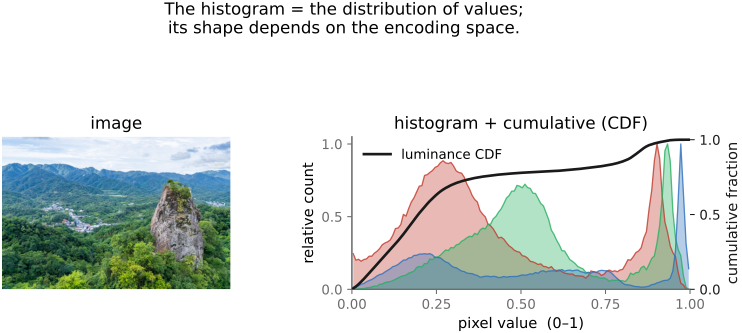
The histogram of an image is the distribution of its pixel values: for each value — or, in practice, each small bin of values — how many pixels carry it (Figure 4.5.1). That is the whole definition. You sweep the value axis from black (0) to white (1), and at each point you plot a count. A grayscale image gives a single curve; a color image gives three, one per channel, usually drawn overlaid.
The striking thing is what the histogram throws away. It keeps no spatial information at all — not where any pixel is, only how many sit at each tone. A face and the sky behind it dissolve into the same pile of counts; shuffle every pixel in the image to a random location and the histogram does not change. That sounds like a catastrophic loss, and for many tasks it is, but for judging exposure it is exactly the right summary, because exposure is a statement about tones, not about places.
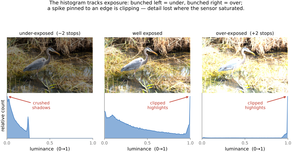
So learn to read it. A glance tells you whether an image uses the full tonal range or wastes part of it. Counts piled hard against the left edge mean crushed shadows — pixels stuck at pure black, their detail gone. Counts piled against the right edge are clipped highlights — pixels saturated at pure white, equally unrecoverable. A spike pinned to either end is the tell-tale of clipping: many distinct scene tones have collapsed onto the same extreme value. A distribution bunched in the middle with empty margins is a low-contrast, flat image that is not using the range it has — the cue to reach for the levels sliders and stretch it out. None of this requires looking at the photograph; the chart says it directly.
The shape of the histogram also tracks exposure directly: change the exposure and the whole distribution slides along the value axis, left for darker, right for brighter, until tones run off an edge and pin there as a clipping spike (Figure 4.5.2). This is the histogram's day job — it is how you confirm an exposure is using the available range without blowing the highlights or crushing the shadows, and it is why every serious camera and editor puts one on screen.
4.5.2 the histogram depends on the encoding space⧉
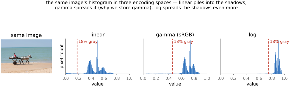
Here is the trap, and it is the reason this chapter insists on it: the shape of a histogram depends entirely on the numerical space the values are stored in. The same image — the same physical scene, the same pixels of light — has a completely different histogram in linear light than in gamma-encoded (sRGB) values than in a log encoding. Nothing about the scene changed; only the ruler we used to measure each pixel did, and the histogram is a picture of that ruler as much as of the scene (Figure 4.5.3).
The reason is that these encodings space the tones differently. Linear values are proportional to physical radiance, and most of a natural scene's pixels are dark — so in linear light the distribution piles into the shadows, bunched near 0, with the bright minority stretched thinly toward 1. A gamma (sRGB) encoding applies a roughly cube-root curve that lifts the darks, which spreads that shadow pile out across the value axis into something far more even — which is exactly why gamma is the encoding we display and edit in. A log encoding spreads the shadows even more aggressively, since equal ratios of light become equal steps.
A concrete landmark: the 18% gray card, the mid-tone a light meter is calibrated to. Its linear-light value is 0.18 — sitting down in the lower fifth of the axis. Apply the sRGB gamma and that same gray lands near 0.46, almost exactly in the middle. In a log encoding it climbs higher still, to roughly 0.75. One physical tone, three completely different positions, purely because of the encoding. So whenever you read a histogram — to judge exposure, to set a black point, to equalize — you must know which space it was computed in, or you will misread it. "The histogram looks dark" is a meaningless statement until you say which histogram.
4.5.3 a histogram is a sampled estimate⧉
One caveat before we put the histogram to work. A histogram is not the true, continuous distribution of the scene's tones — it is a sampled, discretized estimate of it, and that estimate has artifacts you must not mistake for signal. Two effects in particular:
Binning. You chose a finite number of bins (256 is common for 8-bit data), and the bin width sets the resolution. Too few bins smears real structure together; too many leaves the counts noisy and gappy. The comb-like ridges you sometimes see are an artifact of the bin grid, not the scene.
Quantization. If the underlying values are themselves quantized — an 8-bit image has only 256 distinct levels — then the histogram inherits spikes and gaps: tall counts at the levels that exist and empty bins between them. This is especially severe after a stretch (levels or equalization), which spreads 256 input levels across a wider output range and leaves visible combing. Those gaps are an artifact of the quantization, not evidence of anything about the photograph. Read the overall shape — where the mass sits, whether it clips — and do not over-interpret the fine teeth.
4.5.4 histogram equalization⧉
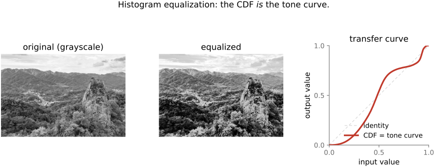
Now the payoff: the histogram is not just a thing to read, it can drive an automatic tone curve. The classic move is histogram equalization, and it rests on one clean idea. Recall the cumulative histogram, or cumulative distribution function (CDF) — the running total of the histogram, swept from black to white, climbing monotonically from 0 to 1. Use that CDF as the tone curve itself:
That is the entire algorithm: build the image's CDF, then push every pixel value through it. Concretely, count the pixels into bins, sweep left to right accumulating a running total, normalize it to climb from 0 to 1, and use the result as a per-pixel look-up table:
hist = zeros(B)                  # B bins over [0, 1]
for each pixel value L in im:
    hist[bin(L)] += 1
cdf[0] = hist[0]
for b in 1 .. B-1:               # running total, left to right
    cdf[b] = cdf[b-1] + hist[b]
cdf = cdf / cdf[B-1]             # normalize to 0 .. 1
for each output pixel (x, y):
    out[x, y] = cdf[bin(im[x, y])]
The result is an image whose own histogram is, as nearly as discretization allows, flat — every tonal bin holds about the same number of pixels (Figure 4.5.4). The reason is intuitive: the CDF is steep wherever pixels are crowded and shallow wherever they are sparse, so it pulls crowded tones apart and squeezes empty stretches together. That is exactly the remap that levels them out. Equalizing maximizes global contrast: it allocates the most output range to the tones the image actually uses most.
It is also a textbook case of everything in this chapter coming together. The CDF is a one-dimensional curve, so equalization is just a point operation — one curve applied to every pixel, computable as a look-up table (LUT) and shippable as one. And because the CDF is computed from the histogram, it depends entirely on the encoding space the histogram was built in: equalize in linear versus gamma and you get different curves and different results, for exactly the reason the previous section labored.
The catch is that equalization has no restraint. It flattens the histogram blindly, with no notion of how much contrast the scene should have, so it routinely over-does it — exaggerating contrast in busy regions, amplifying noise in flat ones (more pixels there means a steeper CDF means more stretch), and producing the harsh, over-cooked look that gives naive equalization its bad name. It is a sledgehammer; the rest of this chapter and the next are about taming it.
4.5.5 histogram matching⧉
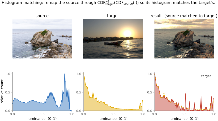
Equalization flattens to a uniform target. But why uniform? Histogram matching (also called histogram specification) generalizes the idea: reshape an image's histogram to match any target distribution you like — a chosen shape, or, more usefully, another image's histogram. You hand it a reference and it makes your image's tonal distribution look like the reference's.
The recipe is elegant: compose two CDFs. First equalize the source — push it through its own cumulative distribution $\text{CDF}_\text{src}$, which (as we just saw) flattens it to a uniform spread. Then un-equalize through the target's inverse CDF, $\text{CDF}_\text{tgt}^{-1}$, which reshapes that uniform spread into the target's distribution. Composed into one curve:
Both pieces are one-dimensional, so their composition is one-dimensional too — matching is still a single point operation, a LUT applied per pixel (Figure 4.5.5). And equalization falls out as the special case where the target is uniform, so $\text{CDF}_\text{tgt}$ is the identity and the formula collapses back to $L_\text{out} = \text{CDF}_\text{src}(L_\text{in})$. Matching, equalization, and a hand-drawn levels curve are therefore one family — all of them one monotone curve on the value axis, differing only in how the curve is chosen.
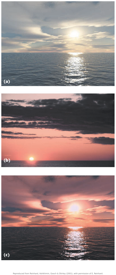
For color, matching needs care. Run the recipe on each of the R, G, B channels independently and you will shift hues — the three channels are not independent, and reshaping them separately moves colors as a side effect. The fixes are to work in a decorrelated or perceptual space where per-channel matching does less damage, or to use a proper multi-dimensional version. The canonical practical method is color transfer (Reinhard, Ashikhmin, Gooch & Shirley 2001): match the mean and standard deviation per channel in the decorrelated $l\alpha\beta$ space — a lightweight statistical match rather than full distributions. The exact N-dimensional version, matching the full joint distribution, is the province of optimal transport (Pitié, Kokaram & Dahyot 2007) — the mass-transport view, in which reshaping one distribution into another is literally the problem of moving "mass" from one histogram to the other at least cost. That framing powers richer edits than plain color transfer: Shu et al. Shu et al. 2017 (portrait lighting transfer) transfer the lighting of a reference portrait onto another by optimally transporting one face's color/tone distribution to match the reference's, so a flatly-lit portrait inherits the modeling of a studio one.
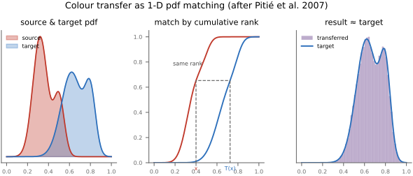
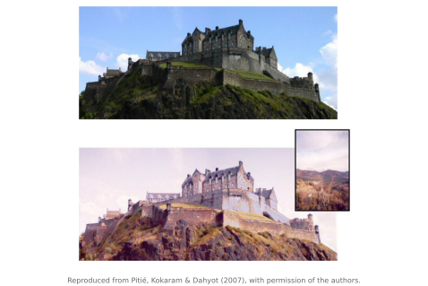
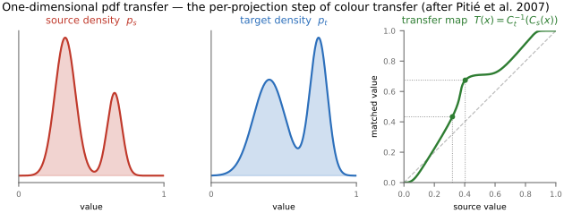
Reinhard's lightweight moment-matching gives much of that payoff for a fraction of the work: shift each channel to the target's mean and scale by the ratio of standard deviations, all in the decorrelated $l\alpha\beta$ space so the per-channel retargeting does not twist the hues — just first- and second-order statistics per channel, yet enough to pour one image's warmth or coolness over another's content. It is the lean ancestor of neural style: first and second moments of raw pixels, where Gatys will later match the second-order statistics of deep features (Reinhard et al. 2001).
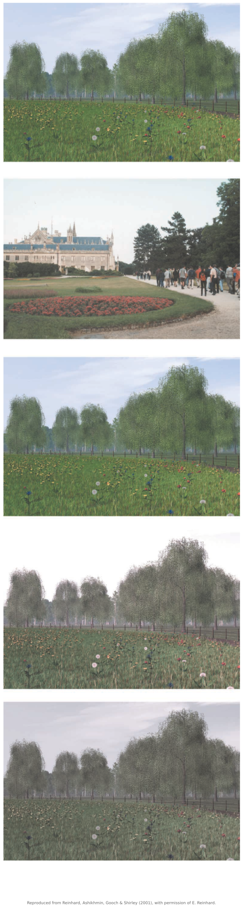
The textbook treatment of the one-dimensional case is Gonzalez & Woods Gonzalez & Woods, Digital Image Processing.
Histogram and color matching turn out to be a workhorse far beyond this chapter. The same "make this image's statistics look like that one's" move powers harmonization (making a pasted region's tones match its new background — see Compositing), color grading and style transfer (imposing a reference look), and even texture synthesis (matching value statistics). It is one of those small ideas that keeps reappearing.
4.5.6 constraining the slope: Ward's histogram-based tone mapping⧉
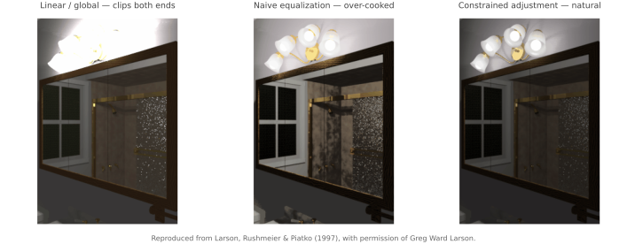
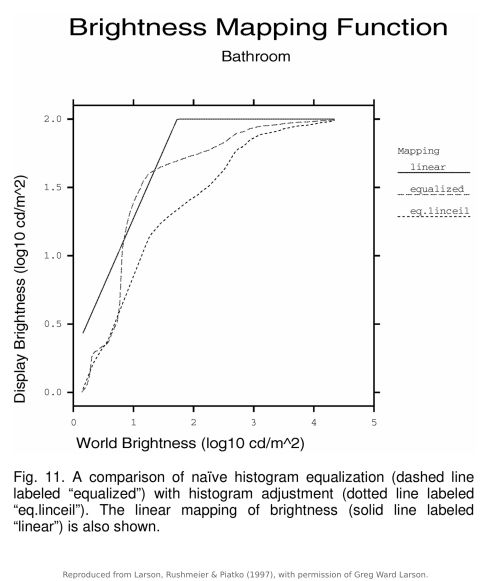
Equalization's flaw — exaggerating contrast wherever pixels happen to crowd — has a clean fix, and it points straight at the next chapter. Greg Ward's constrained, histogram-based tone mapping (Ward, Rushmeier & Piotrowski 1997) keeps the equalization idea but caps the local slope of the transfer curve. The CDF is steep exactly where pixels are dense, and that steepness is what over-stretches contrast there; so Ward's method clamps the slope wherever it would exceed what the eye finds plausible, redistributing the leftover range elsewhere. The result is equalization's data-driven allocation of contrast, but perceptually bounded so it never exaggerates beyond what a viewer accepts.
This matters most for high dynamic range (HDR) imagery, where the whole problem is squeezing an enormous range of scene luminance onto a limited display without either crushing detail or generating cartoonish contrast — and a slope-bounded equalization is a principled, fully automatic way to do it. On Ward's own HDR bathroom test scene the three approaches read side by side (Figure 4.5.11): a plain global curve cannot seat both ends of the range; naive equalization fits the range but over-cooks it; and the slope-capped adjustment keeps equalization's adaptivity without the exaggeration. Overlaying the three transfer curves against scene log-luminance is the whole argument in one plot (Figure 4.5.12). We have arrived at the doorstep of tone mapping, where equalization stops being a histogram trick and becomes one member of a family of curves for fitting the world's light onto a screen. That is the subject of the next chapter; this same Ward operator is revisited in the global-operators recap of Recap tone mapping.