4.1 Image representation⧉
PS1 builds the image class, point operations, and color (YUV, gamma, white balance). → Problem sets (appendix).
The basics of representing images digitally are simple enough to make computational photography easy and fun for beginners: just two-dimensional arrays of red, green, and blue values. However, details matter, and you will save yourself a lot of trouble by paying attention to how exactly images encode information.
4.1.1 An image is an array⧉
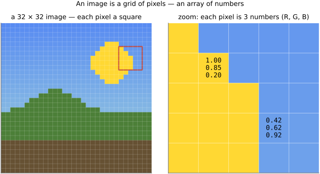
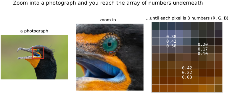
A pixel — short for picture element — is one cell of the grid, and an image is a rectangular array of them. Each pixel holds a short list of numbers describing its color, almost always three: how much red, how much green, how much blue (Figure 1).
It pays to say this a little more formally, because the framing will organize the whole book. An image is a function defined over a 2-D domain, the grid of integer positions $(x, y)$, whose values live in a range, here the space of colors. We store that function as a three-dimensional array of size $\text{height} \times \text{width} \times \text{channels}$ and write $I(x, y, c)$ for the value at column $x$, row $y$, channel $c$. A grayscale image has a single channel, and we drop the index and write $I(x, y)$.
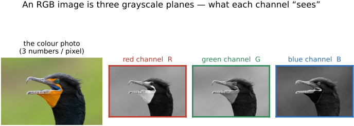
Usually a pixel carries exactly three channels, but nothing forces that. Some images add a fourth — for transparency, which we return to under alpha below — and scientific hyperspectral images keep dozens or hundreds of narrow wavelength bands instead of three broad ones. One very practical trap follows from this freedom, and it bites beginners constantly: a Portable Network Graphics (PNG) file may carry an alpha channel, so a file you assume is three-channel RGB hands you four channels instead. If the rest of your code expects three, every pixel downstream is misread. The fix is trivial once you know to look — check the channel count on load — but the symptom (colors scrambled, code not crashing) is baffling if you do not.
4.1.2 Float vs 8-bit vs more bits⧉
We do our work in floating-point values, and almost always treat the useful range as $[0, 1]$ — $0$ black, $1$ white. The reason is comfort: in float, an image behaves like ordinary numbers. You can add two of them, multiply by a constant, average a hundred, and nothing overflows or quietly truncates to an integer mid-computation. The 8-bit integers ($0$–$255$) you find on disk are excellent for storage and fast hardware, but doing arithmetic directly in 8 bits is a real pain — every intermediate result has to be clamped and rounded, headroom is tiny, and errors accumulate. We confront 8-bit arithmetic squarely in a later chapter; here we simply convert to float on load and back on save, and otherwise forget integers exist.
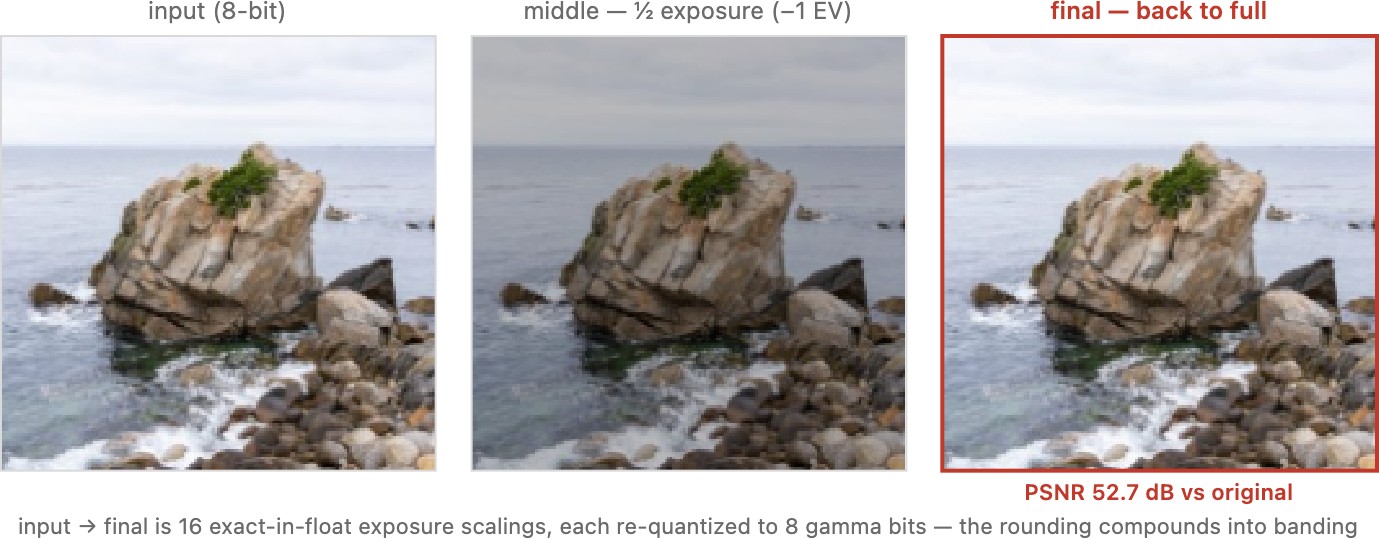
This figure is a deliberate stress test: twenty-odd exposure round-trips through 8-bit storage, on a smooth gradient chosen to band as visibly as possible, built to expose the limit, and it prints the PSNR of the final image against the original so you can watch the damage in numbers. Plain 8-bit holds up better than you might expect: it takes that many compounded round-trips before the degradation is even noticeable, far better than the "only 256 levels!" reflex would predict. Notice, too, how much more resilient gamma encoding is than linear — flip the figure's linear-encoding toggle and the shadows fall apart far sooner, because gamma spends its few code values where the eye needs them (fine steps in the darks, coarse in the bright highlights), so 8 gamma bits go about as far as 12–14 linear bits.
💡 L2.49 — quantization is rarely the real problem (introduced in FUNDAMENTALS → Noise): in a real input file it is noise and dynamic range that limit an image, not the number of discrete levels — which is exactly why floats with headroom are the sane default here, and why a sane encoding (gamma) makes even 8 bits look smooth.
4.1.3 Stochastic Quantization and Dithering⧉
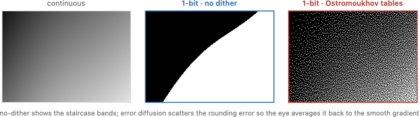
When too few levels force you to round, rounding makes a correlated, structured error — a smooth gradient collapses into flat bands the eye locks onto as false contours. Dithering spends that same error as high-frequency (blue) noise instead, scattering it spatially (a randomized threshold, or error diffusion that pushes each pixel's residual onto its not-yet-visited neighbors) so the local average still tracks the true tone. It works because the visual system integrates noise but sees structure — it low-passes the grain back to the gradient while it would have flagged the bands. The same trade recurs wherever a few levels stand in for a continuum: halftoning in print, coded apertures / masks, computational illumination, blue-noise sampling in rendering, and stochastic rounding in low-precision arithmetic.
When you genuinely cannot afford more bits — a few display levels, a binary mask, a projector with a handful of intensities — the escape from banding is to stop rounding deterministically. The simplest form is stochastic quantization: instead of always snapping to the nearest level, round each pixel up or down at random, with the probability set by where its value sits between the two levels — a value 70% of the way to the upper level goes up 70% of the time. No individual pixel is right, but the expected value is exact, so a patch of constant input becomes a salt-and-pepper mix whose average is the true tone, and the eye — a natural low-pass filter — sees that average instead of a band. This is exactly the stochastic rounding that keeps low-precision (8-bit, fp8) neural-network training unbiased. Its weakness is that it scatters the error with no memory, so it is noisier than necessary — conspicuous white grain.
Error diffusion does better by giving the rounding memory. Floyd–Steinberg's scheme Floyd & Steinberg 1976 still rounds each pixel to the nearest level, but it then pushes the rounding error onto the not-yet-visited neighbors, so the following pixels compensate and the local average tracks the true value with far less noise than random dither. Plain error diffusion leaves directional "worm" textures, which Ostromoukhov's improved algorithm tames by varying the diffusion coefficients with intensity on a serpentine scan, for a cleaner, blue-noise-like result Ostromoukhov 2001 (Figure 4.1.5). One subtlety the figure respects: because the eye averages light, not code values, the quantization and its error must be carried in linear light — only then does the dithered region's average brightness match the original; in gamma/code values the mid-tones come out too bright (Jensen's inequality on the display curve). And both schemes are cleanest at 1 bit (pure black/white, no interior levels to seam); intermediate bit depths leave faint transitions that the variable-coefficient/blue-noise tricks exist to smooth. Crucially, dithering is not just for the display: the same idea — approximate a continuous signal with a few quantized levels by scattering the error spatially — recurs in coded imaging (a binary or few-level aperture/mask standing in for a continuous transmittance) and in computational illumination (a projector or light array with limited levels approximating a smooth lighting pattern), both developed later in the book.
Between those extremes lies a whole ladder of more bits, and it matters in practice. Camera sensors typically deliver 12–14 bits per channel in their RAW files — four to six binary digits more tonal resolution than an 8-bit JPEG — and that extra headroom is exactly what lets you rescue crushed shadows or recover a clipped sky in editing. A great deal of real image processing then happens in 16 bits (16-bit integer, or 16-bit "half" float): enough precision that rounding stays invisible through a long chain of edits, at half the memory of 32-bit float. The rule of thumb is that capture and intermediate work want more bits than the 8 a final display needs — you keep precision where errors would otherwise accumulate, and only quantize down to 8 bits at the very last step, on output.
A float stores a number in binary scientific notation: sign × mantissa × 2^exponent. The exponent slides the binary point, so the same ~24 mantissa bits of a 32-bit float deliver the same relative precision whether the value is $0.001$ or $1000$. A few consequences matter for images:
- Precision is relative — fine near $0$, coarser for large values. That is a good match for linear radiance and high dynamic range (HDR) imaging, where you care about ratios, and roughly for how we perceive light (Weber's law).
- Values outside $[0, 1]$ are fine. A super-white highlight, or the negative lobe of a sharpening filter, is just a number; nothing clamps until you actually output to a display or an 8-bit file. This headroom is a genuine convenience — intermediate results can overshoot and come back.
- $0.1$ is not exact in binary, and adding numbers of very different magnitude loses the low bits (a long running sum of tiny values can drift). Usually negligible for images; occasionally not.
infandNaN(0/0,logof a negative,0 × inf) propagate and silently poison an image — one bad pixel can spread on the next blur. A classic bug; check for them when something goes mysteriously blank.float32is the working default.float16/ half halves memory (used in machine learning and some HDR pipelines) at the cost of precision;float64is rarely worth it for images.- Keep fine data centered near zero. Because precision is relative to magnitude, fine detail riding on a large offset — values clustered in a tight band around a big number, far from the origin — loses its low bits. The canonical illustration is Matt Pharr's note on why renderers work in camera space, not world space: pharr.org/matt/blog/2018/03/02/rendering-in-camera-space. Read it if your high-resolution data is not centered around zero.
4.1.4 How the array sits in memory⧉
The array is two- or three-dimensional, but computer memory is one long line of numbered addresses. Something has to decide how the grid gets flattened into that line, and there is no single right answer. Different ecosystems made different choices, which matters the instant you pass an image between them.
Two decisions combine (Figure 3). The first is the order of the axes. Walking through memory pixel by pixel, do the three channels of one pixel sit side by side — red, green, blue, red, green, blue — or are all the reds stored first, then all the greens, then all the blues? The first is interleaved, or HWC (height, width, channel, with the channel varying fastest); the second is planar, or CHW (the channel varies slowest, each channel a single contiguous plane). NumPy's standard image layout is interleaved HWC; the C++ code in this book stores planar; and PyTorch, which we meet much later for machine learning, wants CHW because that is what its convolutions expect. Concretely, in a planar layout pixel $(x, y, c)$ lives at the flat offset $c\cdot W\cdot H + y\cdot W + x$; interleaved, it is at $(y\cdot W + x)\cdot C + c$. You rarely compute these by hand, but seeing them once makes the point that "the array" is really this index arithmetic — and that $W$, the row length, is the stride that converts a 2-D index into a 1-D one.
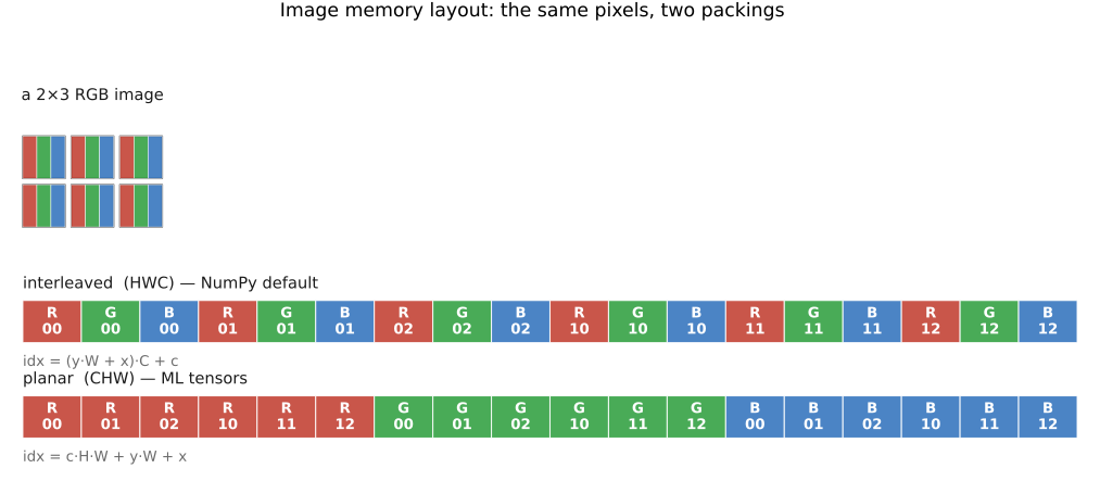
R G B R G B … row by row; pixel $(x, y, c)$ is at offset $(y\cdot W + x)\cdot C + c$. Planar (CHW): all of the red channel, then all of green, then all of blue — three contiguous planes; pixel $(x, y, c)$ is at offset $c\cdot W\cdot H + y\cdot W + x$. Same numbers, same picture; only the walk order through memory differs.The second decision is the order within a pixel. Most of the world, and this book, store the channels as red, green, blue (RGB) — but a few libraries, OpenCV being the notorious one, use BGR. Mix the two and red and blue swap silently: skies turn orange, skin turns blue, and nothing throws an error. So always know which order your data is in.
Why care about any of this for everyday code? Mostly you should not. The mental model is just "a grid of pixels," and the accessor we build below hides the packing entirely. Two situations force you to think about it: performance (a loop that strides through memory in contiguous order runs far faster than one that hops around, so the right layout for an algorithm matters when speed does), and interoperability (handing an image to a library that expects a different layout means rearranging the array first). Outside those, the packing is an implementation detail.
That performance point dictates how you write every loop, so it is worth one more sentence. Memory is fast only when you read it in order: the hardware fetches a whole cache line at a time and prefetches the next, and vector (SIMD) instructions chew through a contiguous run of values in a single step. Both reward walking the array along the direction it is actually stored. For a row-major image the pixels of one row are contiguous, so the loop must put the row index $y$ on the outside and the column index $x$ on the inside — for y: for x: marches straight through memory, cache line after cache line, and vectorizes cleanly. Swap them — for x: for y: — and every step jumps a full row's stride ($W$ values, often several kilobytes) to a fresh, uncached address; the cache thrashes and the identical arithmetic can run several times slower. (Planar layout just extends the rule to three nested loops, channel outermost: for c: for y: for x:.) This is why the data is organized the way it is — not aesthetics, but matching the array's order to how memory and SIMD actually behave — and "is my loop nesting in stride order?" is the first thing to check when an image loop is mysteriously slow. You do not have to take this on faith: the demo below runs both loop orders on a large image in your own browser and times them (Figure 4.1.7).
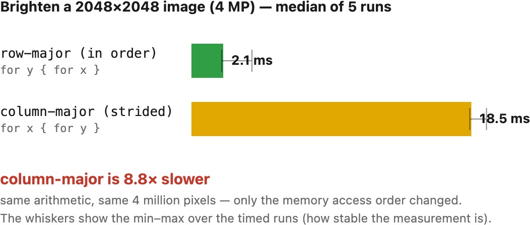
for y { for x } and the cache-hostile for x { for y }, warms up the JIT, then times several passes of each and reports the medians with their min–max spread. The arithmetic and the pixel count are identical; only the memory access order differs, yet the column-major walk typically runs several times slower on the very machine you are reading this on. Interactive: press Run to re-measure, and change the image size; watch the column-major bar stay several times longer than the row-major one, with tight whiskers showing the measurement is stable.The same contiguity argument decides the layout, not just the loop order. A vector unit wants several values of one kind in a row, so a per-channel operation streams cleanly through planar storage, where each channel is a solid block, but stumbles on interleaved R G B triplets, where the reds it wants are scattered every third cell and must be gathered (loading the greens and blues in between only to throw them away). That is a large part of why performance-critical imaging code, and the tensors of machine learning, so often keep the channels planar: packed triplets are convenient to read but hostile to the vector unit.
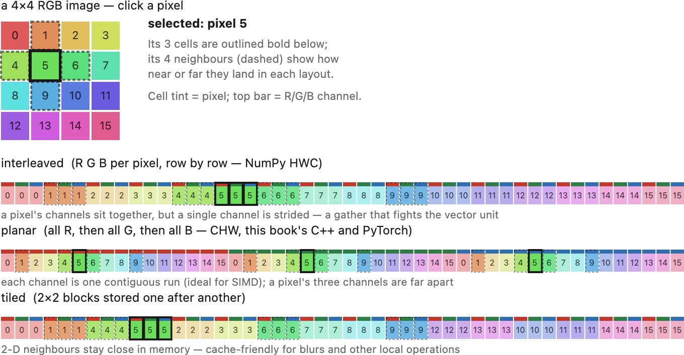
R G B R G B … or as three planar channel-blocks. To brighten the red channel, a 4-wide SIMD load pulls four reds in one contiguous step from planar storage, but must gather them from every third cell under interleaving, touching greens and blues it then discards. Interactive: flip the layout and watch the access pattern change.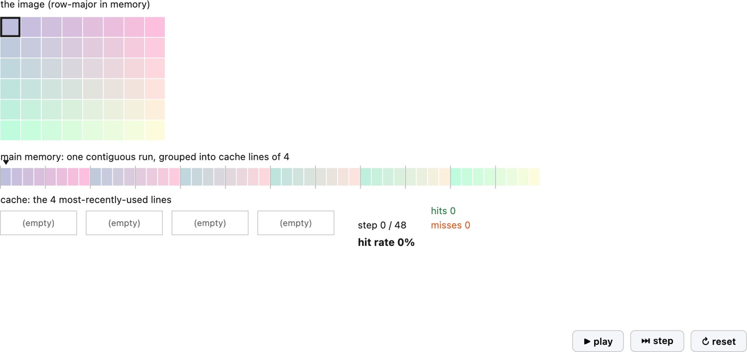
for y { for x } walks memory in order, so each miss loads a line that then serves the next several reads as hits; for x { for y } jumps a full row's stride every step, to a fresh line that is evicted before the loop returns, so almost every read misses. Same pixels, same arithmetic, very different hit rate. Interactive: play or single-step, and flip the loop order to watch the hit rate collapse.Walk an image the way it is laid out in memory. For row-major (HWC) storage that means the inner loop runs over $x$ (columns) and the outer over $y$ (rows) — for y { for x { … } } — so consecutive reads are contiguous, the cache line is used instead of thrashed, and the loop vectorizes. Get the nesting backwards and the identical arithmetic can run several times slower. The rule generalizes: make the innermost loop the fastest-varying index of your actual layout (planar adds channel outermost, for c { for y { for x } }; PyTorch's CHW differs again). It is the humble first instance of the book's performance theme — respect the memory hierarchy — and it returns in earnest in Performance engineering and Halide.
This book carries a concrete, working C++ image data structure, and it is worth seeing once so the planar arithmetic above stops being abstract. It is deliberately minimal — three integers for the shape, and a single flat buffer of floats in planar order:
struct Image {
    int width, height, channels;
    std::vector<float> data;        // planar: c*width*height + y*width + x

    Image(int w, int h, int c)
        : width(w), height(h), channels(c),
          data(static_cast<size_t>(w) * h * c, 0.0f) {}

    // The accessor: hides the index arithmetic, so the rest of the
    // code can think in plain (x, y, c).
    float& operator()(int x, int y, int c) {
        return data[c * width * height + y * width + x];
    }
};
The entire image is one std::vector<float>; pixel $(x, y, c)$ lives at data[cwidthheight + y*width + x] — exactly the planar offset from Figure 3. The operator() accessor buries that formula in one place, so a line like img(x, y, 0) = 1.0f reads as if it indexed a 3-D array even though the storage underneath is flat and planar. (The Python profile of this book uses a NumPy $H \times W \times C$ array instead, indexed arr[y, x, c], which is interleaved HWC — the same image, a different default packing.) We extend this same accessor below to handle out-of-bounds reads, turning it into the single chokepoint through which all pixel access flows.
We store pixel values as floating-point numbers, with $0$ the darkest a channel can be and $1$ the brightest. This keeps the arithmetic sound: adding two images, scaling by a half, or averaging a stack all behave like ordinary numbers, with no overflow or integer rounding to track. Files on disk usually store 8-bit integers ($0$–$255$) for size and speed, and we convert when we load and save. The next section says more about why floats are the right working type — and why values are even allowed to stray outside $[0, 1]$.
4.1.5 Pixel coordinate conventions⧉
Before we trust ourselves to index an image, two small geometric conventions have to be nailed down, because both are silent traps and both differ between tools.
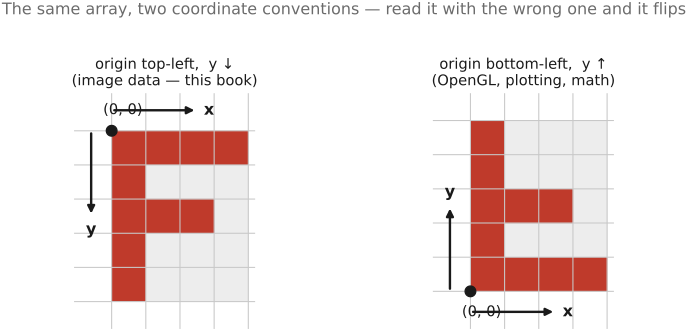
The first is where the origin sits. We place $(0, 0)$ at the top-left pixel, with $x$ increasing to the right and $y$ increasing downward — the order in which image data is scanned and stored, and the convention most imaging code (and our own camera frame) uses. The catch: a few systems — classic OpenGL textures, and much plotting and math software — put the origin at the bottom-left, with $y$ increasing upward, as on a graph. Hand an image from one world to the other without flipping it and the picture comes out upside down (Figure 4.1.10). Nothing crashes; it merely looks wrong, which is the worst kind of bug to chase.
The second convention is subtler and matters more: what an integer coordinate names. A pixel is not a point; it is a little square with area. So does the coordinate $(3, 5)$ refer to the pixel's center or to one of its corners? We adopt the standard choice: integer coordinates name pixel centers. Pixel $(0, 0)$ is centered at $(0, 0)$, so its square spans $x \in [-0.5, 0.5)$, and the continuous image covers $x \in [-0.5,\, W - 0.5)$. The competing convention (integer coordinates at the top-left corner of each pixel, so the image spans $[0, W)$) is also in wide use, and the two differ by exactly half a pixel.
That half-pixel sounds pedantic, and for a point operation it is — a curve applied to every pixel never asks where a pixel is. But the moment you resample or warp — scale up, rotate, correct lens distortion — you are evaluating the image at non-integer positions, and a consistent half-pixel error shifts the whole result by half a pixel, blurs it, or makes a "round trip" (shrink then enlarge) fail to land back where it started. It is one of the most common bugs in resampling code precisely because it never raises an error. We fix the convention now — integer = center — and return to it in full at resampling and warping, where it earns its own discussion of "where-from vs. where-to" addressing.
Keep two facts straight and most coordinate bugs evaporate: the origin is top-left, $y$ down, and an integer coordinate names a pixel's center, not its corner. Both are conventions, not laws — other tools choose differently, so check before you trust.
4.1.6 Alpha and extra channels⧉
So far each pixel has held three numbers, but nothing requires exactly three. The common fourth channel is alpha: a per-pixel opacity (or coverage) value, giving RGBA — how much of this pixel is genuinely "there" versus see-through. Alpha carries one classic pitfall, premultiplied vs straight (whether the RGB values have already been scaled by the alpha), but we do not need it until the compositing chapter Compositing, which treats it in full. The heads-up for now is the narrow, very common one from the array section: load a PNG expecting three channels and you may get four — so check the channel count on load.
Beyond alpha, the array simply gains channels as the task demands. A depth (or Z) channel records distance per pixel; a matte marks out a region; hyperspectral imaging keeps many narrow wavelength bands instead of three broad ones (recall from the light chapter that "color," upstream of the camera, is really a full spectrum — hyperspectral keeps more of it). None of the machinery changes; there are just more numbers per pixel.
4.1.7 Video and more dimensions⧉
Nothing forces us to stop at a flat grid, either. A video is just an image sequence with one extra axis, time: $H \times W \times C \times T$. Most operations we write for a single frame generalize directly — run them frame by frame — and only the operations that couple frames (motion estimation, temporal denoising) need anything new, which we save for the motion and video material.
The same move keeps paying off in other directions. Volumetric imaging stacks 2-D slices into a 3-D block — medical computed tomography (CT) and magnetic resonance imaging (MRI) produce an $H \times W \times D$ volume. A light field adds two angular axes to the two spatial ones (a 4-D record of rays, not just pixels); a spectral cube adds wavelength. In every case it is the same array machinery with more axes. We write this book for 2-D images and point out where adding a dimension is all it takes.
4.1.8 Pixel lookups and boundaries⧉
Almost every operation in the coming chapters reaches for a pixel's neighbors, which forces an unavoidable question: what is $I(x, y)$ when $(x, y)$ lands outside the image? We cannot dodge it, because blurs, gradients, resampling, and warps all ask for out-of-bounds pixels right at the border, where there are no neighbors on one side. Reading past the array is, at best, garbage and, at worst, a crash — so the first discipline is defensive: route every pixel read through a single accessor function, a small get(x, y, c), so that out-of-bounds access is decided in exactly one place rather than re-improvised (and re-broken) in every loop. As a bonus, that one function is also where the memory layout, the channel order, and the coordinate convention live — so the rest of the code can think in plain $(x, y, c)$ and forget every packing decision above. It is the natural home for one more safety check, too: asserting that an index lies in $[0, \text{size})$ inside that single function turns a baffling, far-away crash into an immediate, localized error (we develop this habit in the debugging chapter).
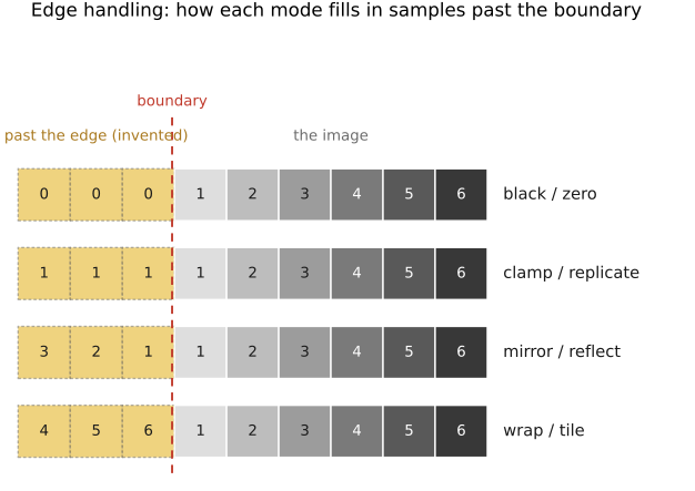
The accessor then has to decide what a pixel past the boundary means. There are four standard policies (Figure 4):
- black / zero — treat everything outside as $0$. Simple, but it darkens edges, since you are averaging in black that is not really there.
- clamp / replicate — repeat the nearest edge pixel outward. A reasonable, neutral default for many operations.
- mirror / reflect — fold the image back across its boundary, so the neighborhood just past the edge mirrors the one just inside. This avoids both the artificial darkening of zero and the streaking of clamp, and is the usual safe default for filtering.
- wrap / tile — treat the image as periodic, the left edge adjacent to the right. Rarely what you want visually, but it is exactly the assumption the Fourier transform makes, so it returns when we get there.
On a real photograph the four policies look like Figure 4b: the same crop, continued past its border each way — surrounded by a dark frame, streaked outward, folded back on itself, or wrapped around from the opposite edge.
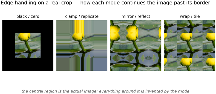
The choice is not cosmetic: it changes what a convolution, a resample, or a warp produces along every border, and a surprising number of "why is there a dark frame / a bright streak around my result?" bugs trace straight back to it. We default to mirror as the safe general choice, fall back to clamp when we want simplicity, and call out wrap wherever Fourier makes it the natural one. With the accessor and its edge policy fixed, the bare grid of numbers we opened with is finally a structure we can compute on — which is exactly what the next chapters do.
4.1.9 Beyond the pixels: basic metadata and EXIF⧉
An image file holds more than the pixel array. Wrapped around it is metadata — data about the data. The most basic metadata describes the array itself: its pixel width and height, the channel count and bit depth, and bookkeeping fields like the file's name and path and its creation date. Some of this you can read straight off the array in memory; the rest the file format records in a header. You will reach for it constantly — width and height set every loop bound, and the channel count is exactly the "three or four?" question from the previous section.
Cameras write a far richer layer of capture metadata into a standardized block called the exchangeable image file format (EXIF). This is where you find the ISO (sensitivity setting), shutter speed, aperture, and focal length the photo was taken at, along with the lens model, a timestamp, often a Global Positioning System (GPS) location, an orientation flag recording which way the camera was held, and an embedded International Color Consortium (ICC) color profile. EXIF is genuinely useful: it is how a photo library sorts by date, plots shots on a map, or auto-rotates a sideways frame.
Treat EXIF as a hint, not a measurement — two things go wrong. First, coverage is incomplete and inconsistent: not every camera writes every field, and the exact set and formatting differ from maker to maker, so any code that reads EXIF has to tolerate missing and oddly-encoded values. Second, and more dangerous, some numbers are only approximate. The recorded ISO and shutter speed in particular are routinely rounded to tidy nominal labels and are not radiometrically correct — they will not let you reconstruct the true exposure, or compare two frames' light, to the precision the digits imply. Do not treat EXIF capture values as calibrated measurements.
A catalog of the fields you will encounter lives in the appendix → Common EXIF fields; the file-format side of metadata — where in the file it sits, and how (or whether) it survives an edit — is in File formats and compression.
A recurring wish in this book: beyond the basics above, a sane image representation would carry exactly the things a bare array can never imply on its own —
- the encoding (linear / gamma / log — the very ambiguity the encoding section below is about);
- the color space / primaries, ideally as an embedded ICC profile;
- the noise level — the read- and shot-noise parameters — so downstream code knows the per-pixel uncertainty it is working with;
- and, when it is known, the point spread function (PSF) — the blur the optics imposed — which is exactly what deblurring needs to undo it.
Most formats carry the first two only unreliably, and the last two not at all. Yet the algorithms that come later silently need this provenance: white balance and HDR want the encoding and color space, denoising wants the noise parameters (see edge-preserving filtering), deblurring wants the PSF. The plain view, then, is that an image is its pixels plus this provenance — and a representation that drops it is forcing every later stage to guess.
4.1.10 Three kinds of operation⧉
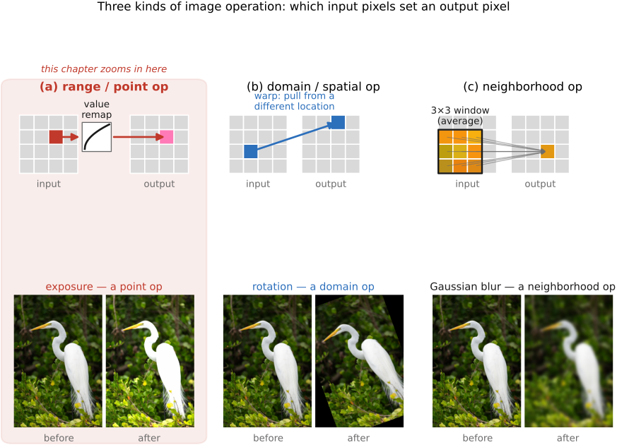
The domain/range split we just drew is not only a definition — it sorts everything we will do to an image into three families, and it is worth naming them now, because the next several chapters are each built around one (Figure 2):
- point operations touch the range only: a pixel's new value depends solely on its old value, the same rule applied everywhere (brightness, contrast, tone curves, gamma);
- domain operations move pixels around without changing their colors: each output pixel pulls its value from a different input location (translation, rotation, resizing, lens correction);
- neighborhood operations compute each pixel from a window of its neighbors (blur, sharpen, edge detection).
This is a preview; each family gets its own development later (point operations come first). But the taxonomy already earns its keep, because it predicts cost: a point operation reads each pixel once, while a neighborhood operation reads many input pixels per output pixel. We will flag which family every new tool belongs to as we go.
Recap: big lessons of this chapter
When too few levels force you to round, rounding makes a correlated, structured error — a smooth gradient collapses into flat bands the eye locks onto as false contours. Dithering spends that same error as high-frequency (blue) noise instead, scattering it spatially (a randomized threshold, or error diffusion that pushes each pixel's residual onto its not-yet-visited neighbors) so the local average still tracks the true tone. It works because the visual system integrates noise but sees structure — it low-passes the grain back to the gradient while it would have flagged the bands. The same trade recurs wherever a few levels stand in for a continuum: halftoning in print, coded apertures / masks, computational illumination, blue-noise sampling in rendering, and stochastic rounding in low-precision arithmetic.
Walk an image the way it is laid out in memory. For row-major (HWC) storage that means the inner loop runs over $x$ (columns) and the outer over $y$ (rows) — for y { for x { … } } — so consecutive reads are contiguous, the cache line is used instead of thrashed, and the loop vectorizes. Get the nesting backwards and the identical arithmetic can run several times slower. The rule generalizes: make the innermost loop the fastest-varying index of your actual layout (planar adds channel outermost, for c { for y { for x } }; PyTorch's CHW differs again). It is the humble first instance of the book's performance theme — respect the memory hierarchy — and it returns in earnest in Performance engineering and Halide.