3.1 Exposure🔗⧉

We have built the physics of image formation: rays selected by a lens, projected by perspective, integrated over the aperture and the pixel and the exposure time, and counted as photons on a sensor. Now we sit behind a real camera and ask the practical questions. Which dial does what, and what does it cost? How does the camera decide the exposure on its own, and when does it get it wrong? How does autofocus find the focus plane, and how does a phone, with a sensor the size of a fingernail and no aperture ring at all, produce a picture that rivals a camera ten times its size? This chapter is the bridge from the abstractions of the previous chapters to the buttons under your thumb, and from there to the computational chapters that make a phone camera work.

The throughline is that every control on a camera is one of the previous chapters made physical. The aperture ring sets the $f/D$ ratio from the lens chapter; the shutter dial sets the exposure time $t$ from the sensor integral; the ISO setting scales the gain that the noise section described; the focus ring moves the image distance $v$ of the thin-lens equation. Learn the physics once and the camera stops being a box of mysterious modes.

3.1.1 Basic photography: exposure settings — shutter, aperture, and ISO🔗⧉

How bright a photo comes out is its exposure, and from the radiometry and sensor chapters we already have the equation: exposure is irradiance times time, and the irradiance the lens delivers scales with aperture area, so

Two optical controls set it. Shutter time $t$ enters linearly: twice the time, twice the light. Aperture enters through its area, which goes as the diameter squared $D^2$, i.e. as $1/N^2$ in the f-number $N = f/D$, so twice the f-number means a quarter the light. This is finally why photographers describe the aperture by the ratio $f/D$ rather than the raw diameter: a longer lens at the same f-number has a proportionally bigger opening, so it gathers the same light per unit of sensor area despite seeing a narrower field of view. The longer lens divides the world into a smaller patch (less light per pixel from the geometry) but compensates with a larger physical aperture (more light gathered), and the ratio $f/D$ is exactly the quantity that nets those two effects out. The ratio normalizes light-gathering across focal lengths, precisely what you want a brightness setting to do.

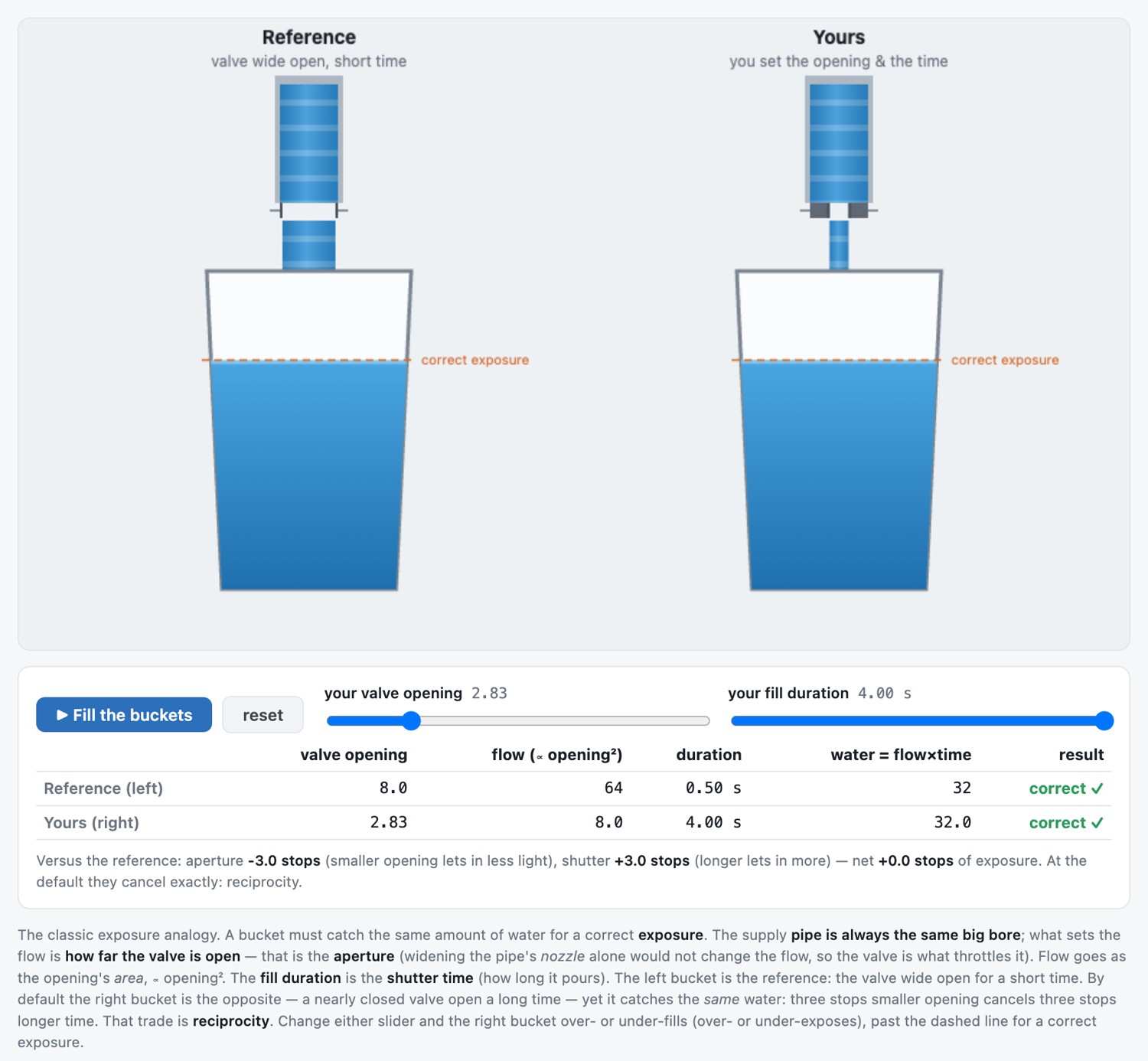
A homely picture makes the aperture-time trade concrete: think of exposure as filling a bucket from a faucet (Figure 3.1.1). The faucet's diameter is the aperture, setting how fast light pours in (the flow follows the opening's area, just as light follows $D^2$), and how long you leave it running is the shutter time. A correct exposure is the bucket filled to the same line however you split the job between the two, so a wide faucet open briefly and a narrow one open a long time can catch exactly the same water. That is why one stop of aperture trades one-for-one against one stop of shutter, the reciprocity the f-number series and shutter series are both built around (below).

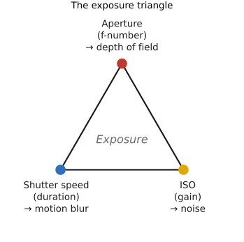
A third control, ISO, is electronic rather than optical: it scales the gain applied to the sensor signal after capture. Raising ISO does not collect more light; it amplifies what was collected, brightening a dim exposure at the cost of also amplifying noise (the sensor chapter's read and shot noise). So the three legs of exposure are shutter, aperture, and ISO: two that change the light and one that changes the gain.

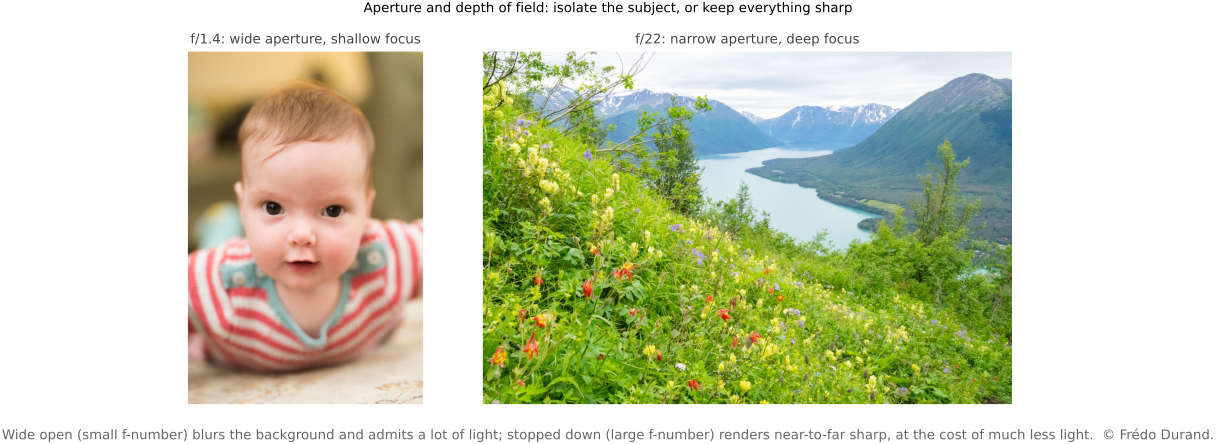
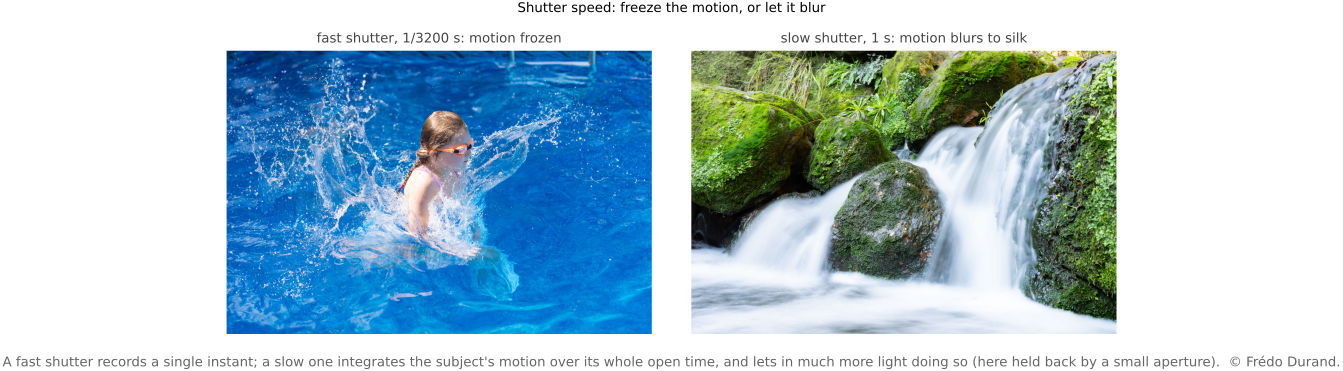
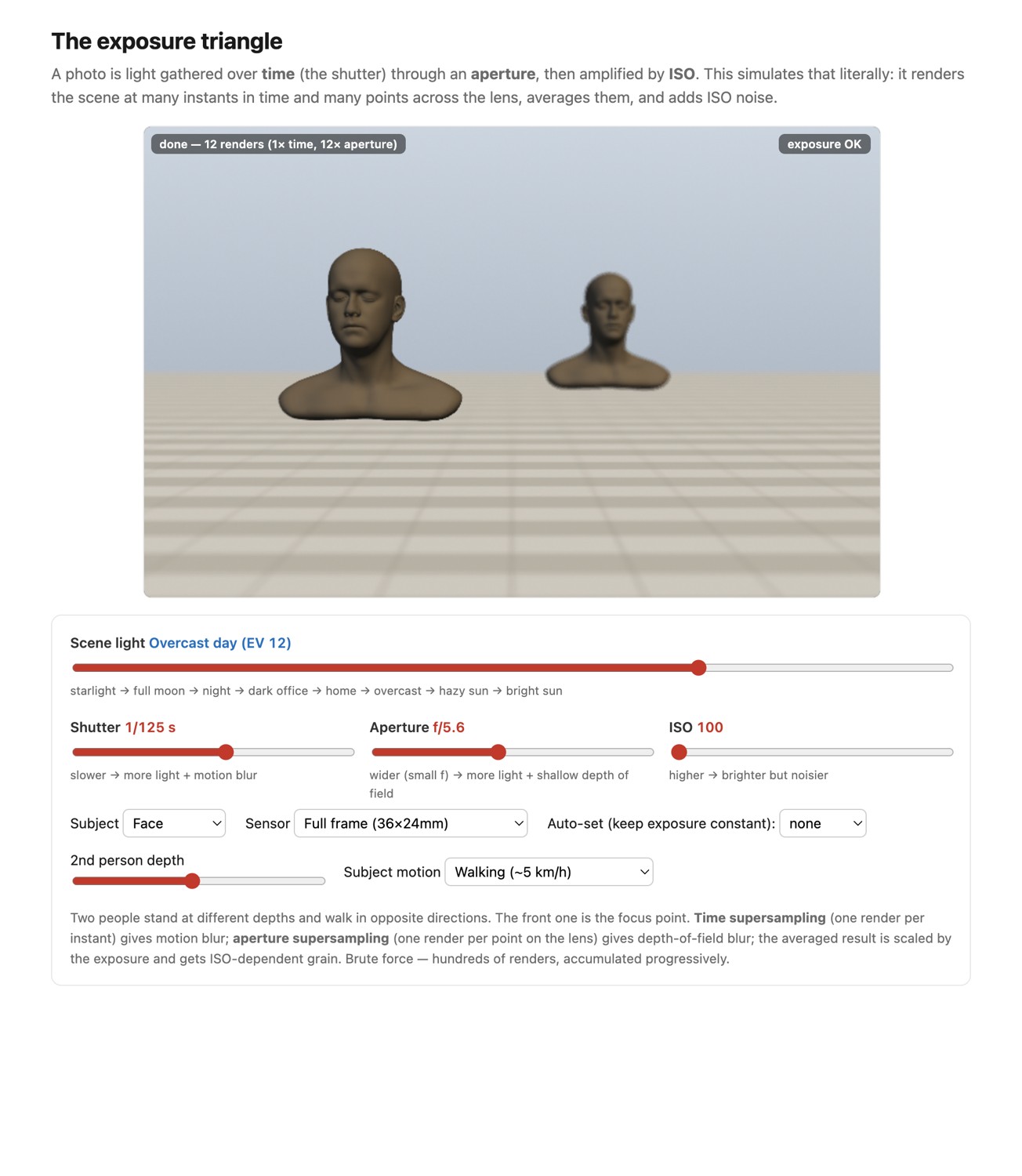
Each control carries a side effect you cannot escape, and each was derived elsewhere in this part. A longer shutter time risks motion blur of anything that moves during the exposure (covered fully in Motion/Video); a wider aperture (smaller $N$) shrinks the depth of field (DoF), the range of distances in acceptable focus (the lens chapter); and a higher ISO raises noise (the sensor chapter). Choosing an exposure means balancing brightness, motion, depth of field, and noise (Figure 3.1.2 and Figure 3.1.3).

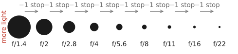
Stops and the power of two. Photographers do not count light in raw multiples; they count it in stops, where one stop is a factor of two in light, the natural unit because the eye and the medium respond to ratios, not differences (the same logarithmic perception behind gamma encoding, in Color technology). One stop brighter is $+1$ exposure value (EV), so a stop is a log₂ unit: $\text{stops} = \log_2(\text{light ratio})$, with $\mathrm{EV} = \log_2(N^2/t)$. This is why the classic f-number series looks so irregular: $f/1.4, f/2, f/2.8, f/4, f/5.6, f/8, f/11, f/16$. Because light $\propto$ aperture area $\propto D^2 \propto 1/N^2$, each step multiplies $N$ by $\sqrt{2}$, so the area, and therefore the light, halves at every step (Figure 3.1.4). Shutter speeds ($1/30, 1/60, 1/125, \dots$ s) and ISO ($100, 200, 400, \dots$) step in the same power-of-two stops; cameras add ⅓-stop clicks for fine control. The point is that one stop of aperture, one stop of shutter, and one stop of ISO all change the brightness by the same factor, so they are interchangeable in exposure calculations, the exposure triangle (Figure 3.1.5).

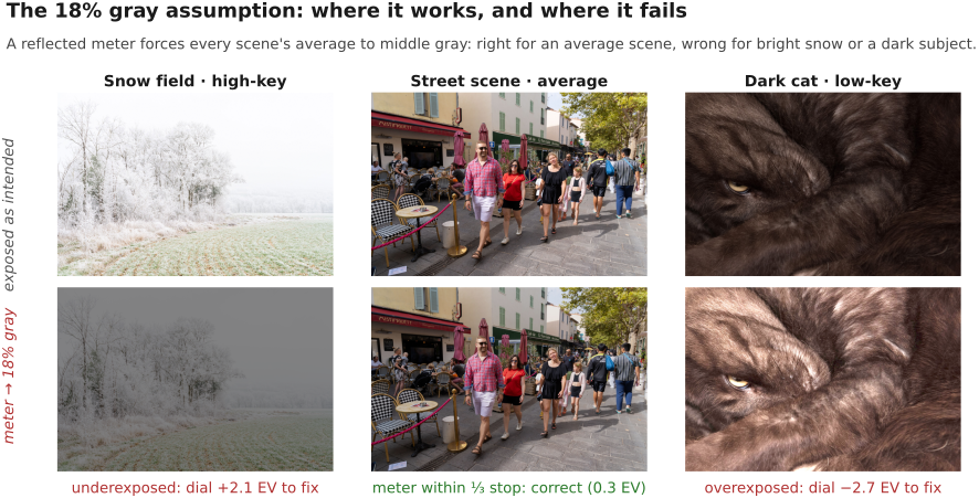
Autoexposure and metering. How does the camera pick an exposure on its own? Its meter integrates the scene's light through the lens (TTL, through-the-lens), as a center-weighted average, a narrow spot, or a smart evaluative/matrix reading, and then renders that average to a mid-gray assumption: it assumes the average scene reflects about 18% gray and sets the exposure to make it so. This works for ordinary scenes and fails predictably on high- and low-key ones (Figure 3.1.7). A snowfield is far brighter than 18% gray, so the meter, dragging it down to gray, underexposes; the snow comes out dingy, and you must dial in $+1$ or $+2$ EV to put it back. A black cat fills the frame with something far darker than gray, so the meter overexposes it to muddy gray, and you dial in $-$EV. Smart matrix metering (Nikon's 3D Color Matrix, learned from a database of tens of thousands of photographs) adds brightness, color, contrast, and distance cues to guess the photographer's intent, but metering remains, in essence, an open problem.

Priority modes. Because shutter and aperture trade off, cameras offer priority modes: in aperture priority you set $N$ (and thus depth of field) and the camera picks the shutter $t$; in shutter priority you set $t$ (and thus motion blur) and the camera picks $N$. Aperture priority is the usual default, because depth of field is usually the creative variable. Each mode fails when no valid partner exists: ask for $f/1.4$ in blazing sun and the required shutter may be faster than the camera can go; ask for $1/1000$ s in a dim room and no aperture is wide enough. (The full mode dial gets its own section next.)

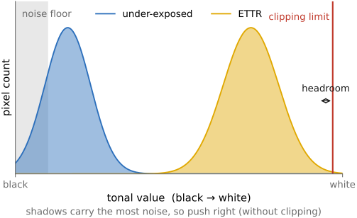
Expose to the right. A subtle but important habit, which the noise section justifies: expose to the right (ETTR): push the exposure as bright as you can without clipping the highlights, so the histogram piles up toward the right edge (Figure 3.1.8). The reason is that noise lives in the shadows (the signal-to-noise ratio is worst where photons are fewest), so capturing more light everywhere, especially in the darks, improves quality; you pull the brightness back down later in software at no cost. And when you do need to brighten, raising the ISO in-camera beats brightening in software, because ISO gain amplifies the signal together with the early (pre-amplifier) noise but not the later read noise added on readout — so the signal gets a head start over part of the noise. ETTR and ISO are both the noise section's logic applied at capture time.

3.1.2 Metering: from printed guides to the sensor🔗⧉

The paragraph above described how a modern meter reasons (render the average to mid-gray) and where it fails. It is worth a moment on how cameras came to meter at all, because the history is a small parable of a measurement being pushed steadily closer to the light it is trying to measure. The full treatment of automatic exposure, including how the camera turns a meter reading into a shutter/aperture/ISO choice, belongs to a later chapter (Auto-exposure and auto white balance); here we only sketch the hardware lineage.

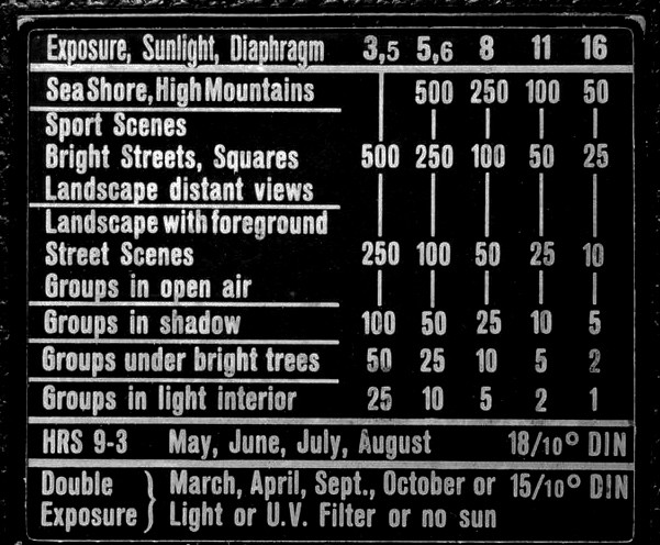
At first there was no meter, only a table. Film came rated for a given sensitivity, and the photographer read the exposure off a printed guide: bright sun, hazy sun, cloudy, open shade, each paired with an aperture and shutter for that film. The guides were everywhere, printed inside the film box, on a slip of paper in the package, on a rotating cardboard exposure calculator, and often engraved on a plate on the camera itself (Figure 3.1.9). The distilled folk version survives as the sunny 16 rule: in bright sun, set the aperture to $f/16$ and the shutter to the reciprocal of the film speed (ISO 100 → $1/100$ s), then open up a stop per step as the light dims. It is metering with no instrument at all, just a lookup table for the handful of lighting conditions the world usually offers.

Then came the instrument. Selenium and later cadmium-sulfide (CdS) and silicon photocells turned incident or reflected light into a needle reading, first in a separate handheld meter the photographer pointed at the scene (or at an incident dome held at the subject), then in a meter clipped onto or built into the camera body, its cell staring out the front. The catch was that a body-mounted cell does not see what the lens sees: change the lens, zoom, or add a filter, and the meter and the film disagree. The fix was to move the cell behind the lens: through-the-lens (TTL) metering, which measures the very light that will expose the frame. In the single-lens reflex (SLR, and later the digital DSLR) this was elegant, because the reflex mirror already diverts the imaging light up to the viewfinder; a cell placed in the pentaprism or aimed at the mirror/focusing screen meters that same beam. TTL is what makes the f-stop-versus-T-stop distinction of the next section invisible for stills: the meter reads transmitted light directly, so lens losses are already in the number.

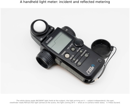
Cutting across this whole evolution is a distinction in what the cell measures, and it still matters today (Figure 3.1.10). A reflected-light meter is aimed at the scene and reads the light coming off it. That is convenient — you can meter from the camera position, and every in-camera meter works this way — but it is subject-dependent: because the meter renders whatever it sees to mid-gray (the 18% assumption above), a snowfield reads too dark and a black cat too light, and you must compensate. An incident-light meter instead carries a translucent white dome that is held at the subject and pointed back toward the camera, integrating the light arriving on the subject over a hemisphere. It never sees the subject's reflectance at all, so it sidesteps the 18%-gray guess entirely and gives the "correct" exposure for a mid-tone directly — which is why studio, portrait, and film photographers reach for a handheld incident meter. This is, at bottom, yet another case of the same asymmetry the visual system is built around: what we care about is the subject's reflectance, not the illumination on it (Human Vision#Lightness constancy). By metering the incoming light rather than the light coming off the subject, the photographer can discount that illumination just as the eye does, pinning the exposure to the light alone so a surface renders to the same tone whether it sits in sun or shade. The catch is practical: you have to physically stand at the subject to take the reading, so incident metering suits controlled setups, while reflected/TTL metering wins for run-and-gun and anything you cannot walk up to. Many handheld meters do both, with a retractable dome for incident and a narrow spot finder for reflected.

The mirrorless era closes the loop entirely. With no mirror and no separate metering cell, the imaging sensor itself is the meter: the camera reads the live scene off the same photosites that will record it, computes a histogram of the actual capture, and previews the exposure in the electronic viewfinder before the shutter ever fires. The measurement and the measured are now the same device. Everything hard about metering that remains, deciding what a "correct" exposure means for a given scene and intent, is no longer a hardware problem but an inference problem, which is where computational auto-exposure takes over (see Auto-exposure and auto white balance).

3.1.3 f-stops versus T-stops🔗⧉

The f-number is a purely geometric quantity: $N = f/D$, focal length over entrance-pupil diameter, and nothing else. It predicts the light a perfect, lossless lens would gather. Real lenses are not lossless. Every air-to-glass surface reflects a little light back (about 4% uncoated, cut to a few tenths of a percent by modern multicoatings), the glass itself absorbs a little, and the barrel vignettes the corners. A simple prime with a handful of elements loses only a few percent, but a big zoom with fifteen or twenty elements can swallow a third of a stop to a full stop before any light reaches the sensor. Two lenses set to the same f-number can therefore deliver visibly different exposures.

The T-stop (transmission stop) folds those losses in. It is the f-number of an ideal lossless lens that would pass the same amount of light, so it is measured on a bench, not computed from geometry:

where $\tau \in (0,1]$ is the lens's transmittance. Because $\tau \le 1$, the T-stop is always a little slower (a higher number) than the f-stop: a lens engraved $f/2.0$ might test at $T/2.3$.

Which number you reach for depends on what you are computing, because a lens carries both. Depth of field is set by the f-number, since the blur geometry (the circle of confusion of the depth-of-field discussion) depends on the physical aperture diameter, which coatings and reflections do not change. Brightness is set by the T-stop, since that is the light that actually reaches the sensor. Two questions, two numbers, one lens.

For stills this distinction is mostly invisible: the camera meters through the lens (TTL), so autoexposure already measures the transmitted light and silently compensates for whatever the lens loses. You can shoot a whole career reading only f-numbers. Cinema is different. A film is cut together from shots made on many different lenses, and a colorist expects every shot taken at a given stop to have matched exposure, so the crew sets exposure from an external meter against the marked stop. Were the marks f-numbers, swapping a clean prime for a heavy zoom at the "same" aperture would jump the exposure and break the match. So cinema lenses are engraved in T-stops instead, calibrated per lens, and a T/2.8 on the 24 mm passes exactly as much light as a T/2.8 on the 85 mm. It is one of several ways cinema glass is built to a different specification, taken up under Video.

Even the T-stop tells only the on-axis story. Off-axis, brightness falls toward the corners: this is vignetting, and it comes in two flavors. Natural vignetting is pure geometry: an off-axis patch of sensor sees the aperture foreshortened into an ellipse, farther away and tilted, so less of it collects less light. For a simple lens the falloff follows the famous $\cos^4\theta$ law, where $\theta$ is the angle off the optical axis, which is why wide-angle lenses (large $\theta$ at the edges) darken corners the most. Optical and mechanical vignetting adds to it: the rims of the barrel and of the other elements physically clip the oblique light cone, an effect worst wide open and one that stopping down a stop or two largely cures. The upshot for photometry is that the effective aperture, and therefore the exposure, is a function of position in the frame, not a single number. Cameras hide this with a built-in flat-field correction (a per-lens brightness map applied in the pipeline), and raw converters carry vignetting profiles, but the correction brightens the corners by amplifying their signal, and with it their noise. So vignetting is not only a brightness artifact; it is one more reason the single f-number or T-stop on the barrel is an idealization, as the next section spells out.

3.1.4 From exposure to photometry🔗⧉

The three exposure controls are, at bottom, a measurement of the scene: fix the geometry and you can read scene light off the settings, and settings off the scene light. This section closes the loop between the photographer's units (an f-number, a shutter time, an ISO) and the physicist's units (radiance, illuminance, and a raw count of photons), building on the radiometric-versus-photometric discussion of the light chapter (Radiometric versus photometric units). Two warnings at the end explain why the answer is only ever an estimate.

Settings to scene luminance. A reflected-light meter is calibrated so that a given scene luminance $L$ (in cd/m$^2$) calls for a definite combination of aperture, shutter, and speed. The ISO metering standard writes this as

where $N$ is the f-number, $t$ the exposure time in seconds, $S$ the ISO arithmetic speed, and $K$ the reflected-light calibration constant ($K \approx 12.5$ for most makers, some use 14). Solving for the scene,

So the settings alone estimate the scene luminance. Sunny 16 is exactly this equation: $N=16$, $t=1/100$ s, $S=100$ gives $L = 12.5\cdot 256 / (0.01\cdot 100) \approx 3200$ cd/m$^2$, the luminance of a mid-gray card in full sun. The estimate is only as good as the "average scene is mid-gray" assumption behind $K$, which is why the metering caveats above apply.

Scene to the sensor. The light actually landing on the sensor is the image-plane illuminance. For a subject far compared with the focal length,

with $\tau$ the lens transmittance (the T-stop correction) and the $\cos^4\theta$ factor the natural vignetting toward the frame edge. The dose of light delivered over the exposure, the photometric exposure or light dose, is

ISO speed is defined through this dose: the saturation-based speed is $S_\text{sat} = 78 / H_\text{sat}$, so at ISO 100 the sensor clips at $H_\text{sat} = 0.78$ lux$\cdot$s. Our sunlit mid-gray, with $\tau\approx0.9$ and $\theta\approx0$, gives $E = \tfrac{\pi}{4}\cdot0.9\cdot3200/256 \approx 8.8$ lux and $H = 8.8\cdot0.01 \approx 0.088$ lux$\cdot$s, about three stops below clipping, right where a mid-gray belongs.

Photometric to radiometric to photons. Photometric units are radiometric units weighted by the eye's luminous-efficiency curve, so converting back requires dividing by the luminous efficacy $K_\lambda$ (lm/W) of the scene's spectrum. At the 555 nm peak $K_\lambda = 683$ lm/W; for broadband reflected daylight it is more like 250 to 350 lm/W, and it genuinely depends on the spectrum, which is the first place real numbers get soft. The radiant exposure at the sensor is then $H_e = H / K_\lambda$ (J/m$^2$). Finally, each photon carries energy $hc/\bar\lambda \approx 3.6\times10^{-19}$ J at $\bar\lambda \approx 555$ nm, so the photon count per unit area is $H_e\,\bar\lambda/(hc)$, and the photons landing on one photosite of pitch $p$ are

Run the sunlit mid-gray through with $K_\lambda \approx 300$ lm/W and a $p = 4\ \mu$m pixel: $H_e \approx 0.088/300 \approx 2.9\times10^{-4}$ J/m$^2$, a photon areal density near $8\times10^{14}$ /m$^2$, and about $1\times10^{4}$ photons in the pixel over the exposure (fewer still turn into electrons, by the quantum efficiency $\eta \approx 0.7$). That a daylit mid-gray delivers only tens of thousands of photons to a small pixel, and far fewer to a phone's sub-micron one, is the whole reason computational photography exists: the shot-noise budget of the sensors chapter (Sensors) is set right here, at the photon count these equations produce.

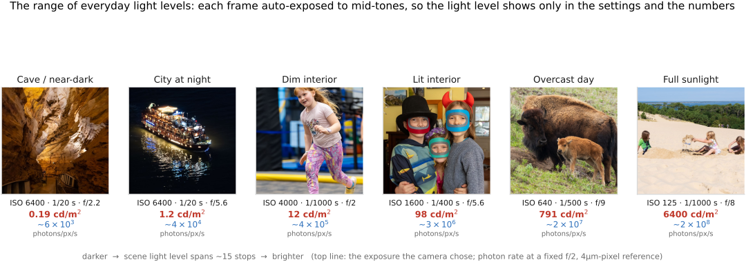
Run the same chain across a range of scenes and you feel just how wide the working range of a camera is (Figure 3.1.11). Six ordinary photographs, from a near-dark cave to full sun, span more than four decades of scene luminance, roughly fifteen stops, yet they all look about equally bright, because each was auto-exposed to mid-tones. The light level is invisible in the picture and shows only in the numbers: the exposure triangle the camera actually chose (ISO, shutter, aperture), the scene luminance those settings imply in cd/m$^2$ (through $L = KN^2/(tS)$, the meter's own relation), and, beside it, the photon rate that luminance implies at a fixed reference. That rate is what everything downstream must live within: the near-dark end delivers a few thousand photons per pixel per second and is firmly noise-limited, while the sunlit end delivers hundreds of millions and is not. The exposure controls exist to slide that photon budget onto the sensor's usable range.

Warning 1: the reported numbers are nominal. Plugging EXIF values into these formulas gives an estimate good to perhaps a third to half a stop, not a calibration. The marked ISO is a manufacturer's choice with real latitude, and the standards even allow different definitions (a saturation-based speed versus a recommended exposure index), so two bodies "at ISO 100" can differ. Marked shutter times are nominal ($1/100$ s may really be $1/96$), and marked f-numbers are rounded to the standard scale. Treat the settings as a good guess at the light, not a measurement of it.

Warning 2: f-numbers and vignetting are subtle. As the previous two sections showed, the geometric f-number is not the transmitted-light number (that is the T-stop, $N/\sqrt\tau$), the working aperture is larger than the marked one at close focus (the effective f-number is $N_\text{eff} = N(1+m)$ for magnification $m$, the bellows factor), and vignetting makes the effective aperture, and therefore $E$ and $n_\text{photons}$, a function of position in the frame through that $\cos^4\theta$ term and the mechanical cutoff on top of it. There is no single $N$ that is correct across the whole image, which is exactly why the exposure a raw file records and the exposure these equations predict never quite agree.

3.1.5 Exposure modes, UI, and auto-ISO🔗⧉

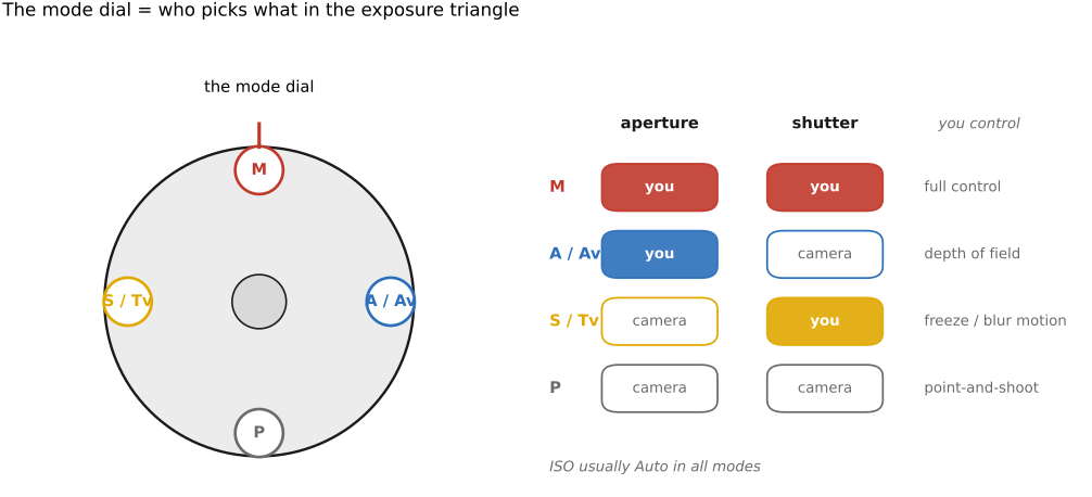
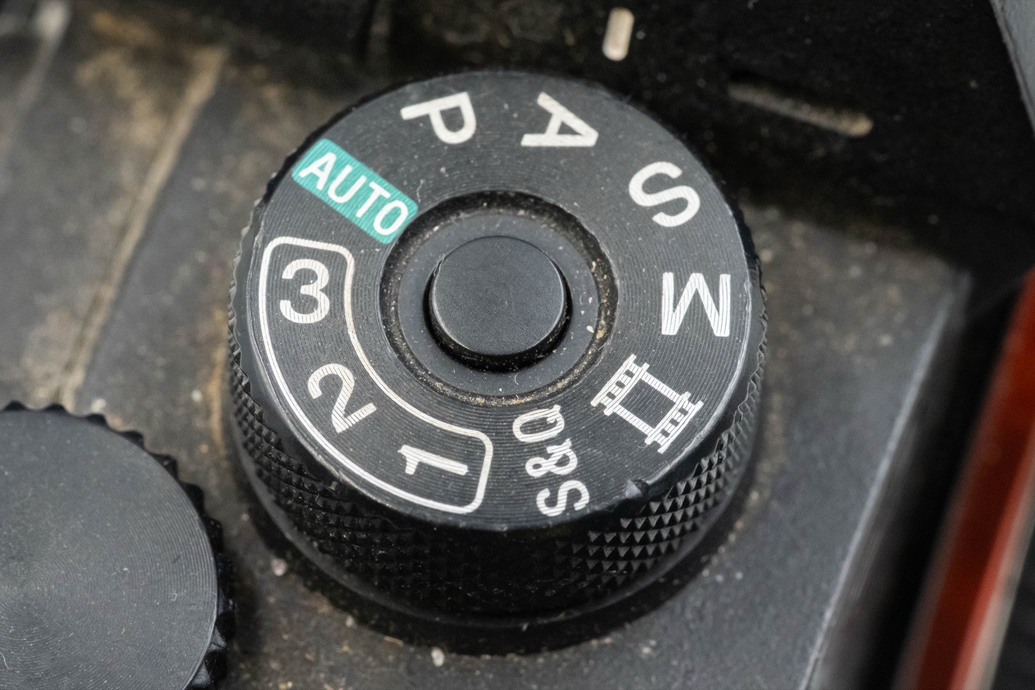
The mode dial looks complicated, but underneath it is just who picks which leg of the exposure triangle. The four classic program, aperture-priority, shutter-priority, and manual (PASM) modes are exactly the four answers (Figure 3.1.12):

• P (program): the camera picks both aperture and shutter from the meter, and you can "program-shift" to slide along the equally-exposed pairs (more aperture, faster shutter, and vice versa).
• A / Av (aperture priority): you set the aperture (and thus the depth of field), the camera picks the shutter.
• S / Tv (shutter priority): you set the shutter (and thus the motion rendering), the camera picks the aperture.
• M (manual): you set both, and the meter only advises.

Beyond these sit full Auto and the scene modes (portrait, sports, night), which are presets that bias the program toward a guessed intent.

Auto-ISO is the modern fourth knob, and it changes the logic. In plain A or S the camera still has only one free leg, so a single setting can over- or under-expose when the light is extreme. Auto-ISO frees a second leg by letting ISO float: now you can hold both a chosen aperture and a minimum shutter speed, and let the ISO climb to make the exposure work. You cap the maximum ISO (your noise budget) and a minimum shutter speed, often a "1/focal-length" rule (so a 200 mm lens won't drop below 1/200 s) or a multiple of it. This is why M + auto-ISO has become a popular combo: you nail aperture and shutter for the look you want, and let ISO be the automatic variable, with exposure compensation still steering it.

Exposure compensation (±EV) is the manual override for the meter's 18%-gray failure without leaving an auto mode: it biases the mid-gray target, so a snow scene gets $+$EV and a dark scene $-$EV. On a mirrorless body the dedicated dial and the live exposure meter make this immediate: you see the brightness change before you press the shutter, the subject of the UI and display section below.