2.15 Imaging as an inverse problem⧉
Two chapters ago we learned what a camera does: it takes the scene, applies a linear operator, and writes down the result: $\mathbf{y}=A\mathbf{x}$. One chapter ago we learned that the sensor does not write it down cleanly: it adds noise. Put the two facts on one line and you have the equation that organizes much of the rest of the book: the fundamental equation of imaging:
Here $\mathbf{x}$ is the scene or image we actually want, $A$ is the imaging operator (a blur, a projection, a sub-sampling, a mask) and $\mathbf{n}$ is noise. Reading the equation left to right is the forward direction: it describes what the camera produced, and the previous two chapters taught us to understand it completely. This chapter is about reading it right to left: given the measurement $\mathbf{y}$, and some model of $A$, recover $\mathbf{x}$. That is the inverse problem, and it underlies most restoration tasks in the book. Deblurring, super-resolution, demosaicking, inpainting, denoising, tomographic reconstruction, refocusing a light field, depth from defocus: every one of them is this same equation solved backward, with nothing changed but the operator $A$ (Figure 2.15.1).
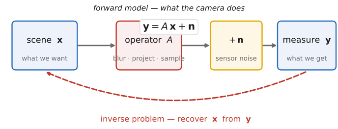
The reason the backward direction is hard (and it is genuinely hard, not merely tedious) is that information is lost on the way down, in two separate ways. The first is the noise: the $+\mathbf{n}$ term means that even a perfectly invertible $A$ hands back a corrupted answer, because we are inverting $\mathbf{y}$, not the clean $A\mathbf{x}$. The second is the operator itself: a real $A$ is almost never a clean, invertible square matrix. It can be rectangular (fewer measurements than unknowns) in which case it literally throws scene degrees of freedom away; or it can be square but ill-conditioned: it squashes some components of the scene almost to zero, so that undoing it means dividing by almost nothing, which detonates whatever noise was sitting there. Either way, the naive instinct ("just multiply by $A^{-1}$") is a catastrophe.
Inverting $\mathbf{y}=A\mathbf{x}+\mathbf{n}$ is hard for exactly two reasons: the operator and the noise. The noise $\mathbf{n}$ corrupts every measurement, so even a perfectly invertible $A$ hands back a corrupted answer. And the operator $A$ throws information away: it can be rectangular (fewer measurements than unknowns, as in the Bayer mosaic, which records only one color channel per pixel) or ill-conditioned: technically invertible but crushing some directions of the scene almost to zero, as in the blur from camera shake, so undoing it divides by almost nothing and detonates the noise. Two further twists make it worse: sometimes $A$ is itself unknown and must be estimated alongside the scene (blind deblurring), and even when it is nominally known, modeling $A$ precisely is hard: a subtly wrong operator yields confident artifacts. Everything downstream in this chapter is the fight against these.
There is a precise word for this kind of trouble. Following Hadamard, a problem is well-posed if a solution exists, is unique, and depends continuously on the data Hadamard 1902. Imaging inverse problems routinely violate all three: noise means no $\mathbf{x}$ exactly reproduces $\mathbf{y}$; a null space means many scenes reproduce it equally; and ill-conditioning means a hair of measurement noise can swing the naive estimate wildly. A problem that fails these tests is ill-posed, and the central fact of this chapter is that an ill-posed problem cannot be solved by cleverness alone: it can only be solved by bringing in extra knowledge about what $\mathbf{x}$ is allowed to look like. The rest of the chapter is two ways of supplying that knowledge, and what the knowledge actually is.
Those two ways are two perspectives on the same act, and they will turn out to be the same perspective in disguise. The first is the linear-algebra view: treat recovery as a least-squares fit, notice that it misbehaves, and regularize it: add a penalty that discourages implausible answers. The second is the probabilistic, Bayesian view: write down how likely the measurement is for each candidate scene (the likelihood), multiply by how likely each scene is a priori (the prior), and pick the best. The result, which we will reach in both formulations, is that when the noise is Gaussian and the observation is linear, regularized least squares and Bayesian estimation with a Gaussian prior are exactly the same equation: you reach one from the other by taking a logarithm. The Bayesian frame is the more general and the more candid of the two, because it names where the extra knowledge comes from: the statistics of natural images, which is the first thing this chapter takes up.
2.15.1 Linear algebra: how hard is this problem?⧉
Before trying to invert anything, the linear-algebra view asks a blunt and useful question: look at $A$ and predict how badly it is going to behave. Two properties tell you almost everything: the operator's shape and its conditioning (Figure 2.15.3).
Start with shape, because it decides whether the problem is even determined (Figure 2.15.2). If $A$ is square and full-rank, there are as many measurements as unknowns and the system is, in principle, solvable, though "in principle" is doing real work, as we will see. If $A$ is tall (more measurements than unknowns, as when you shoot a burst of frames of the same scene) the system is overdetermined: no single $\mathbf{x}$ threads all the noisy measurements, but the least-squares solution $\hat{\mathbf{x}}=\arg\min_{\mathbf{x}}\lVert A\mathbf{x}-\mathbf{y}\rVert^2$ averages the noise down, and more frames give a cleaner answer. This is the happiest case, and it is exactly why multi-shot methods work (11 Multiple exposure imaging). The harder case is the opposite: a wide $A$ (fewer measurements than unknowns, as in super-resolution, inpainting, or demosaicking) is underdetermined, and it has a null space: an entire subspace of scenes that the operator maps to the same measurement. Demosaicking is a vivid everyday example: a Bayer mosaic records just one color channel at each pixel, so for a full-color image two of every three color values are never measured at all: fully two-thirds of the rows we would need are missing, and the camera fills them in (demosaicks) only by leaning on a prior about how colors and edges behave. The data, by itself, cannot choose among them. No amount of computation extracts an answer the measurements do not contain; something outside the data has to break the tie. This is the first place a prior stops being optional.
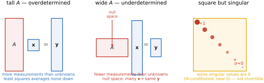
Before the general case, look at the easy one, because it organizes everything that follows: $A$ square and diagonal. Then the equation decouples completely (each measurement is just one unknown times one diagonal entry, $y_i = a_{ii}\,x_i + n_i$) and inverting is nothing but per-element division, $x_i = y_i / a_{ii}$. You can read the trouble straight off the diagonal: wherever an entry $a_{ii}$ is large the inversion is gentle, and wherever it is near zero the division blows the noise up. No subspaces, no entanglement, just a list of independent gains. This case matters because many operators can be made diagonal by a change of basis. For the convolutions that dominate imaging (blur, defocus, motion) the Fourier basis does exactly this (each frequency is rescaled on its own; → the BASICS chapter on Fourier), turning deblurring into per-frequency division and ill-conditioning into simply the frequencies the blur zeroed out. Diagonalizable operators are the ones we truly understand.
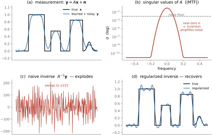
Now conditioning, which is subtler and where most of the real pain lives, because even a square, technically invertible $A$ can be useless. The plain way to see a general operator (one no single change of basis diagonalizes) is through its singular values: the set of gains $\sigma$ by which it stretches or shrinks the different directions of the scene, the diagonal case's "gains" generalized to any matrix. Inverting $A$ means multiplying each direction by $1/\sigma$. If the singular values run from large down to nearly zero (a large condition number $\kappa(A)=\sigma_{\max}/\sigma_{\min}$) then the directions with tiny $\sigma$ get multiplied by an enormous $1/\sigma$, and any noise that happened to land on those directions is amplified without mercy. A lens blur is the textbook villain: it attenuates high spatial frequencies almost to nothing (tiny singular values up there), so naive deblurring divides the noisy high frequencies by almost zero and the image dissolves into a blizzard. Figure 2.15.3 shows this in one dimension, and it is the picture to keep: the true signal, blurred and lightly noised; the operator's singular values sliding toward the noise floor; the naive inverse exploding into garbage; and a regularized inverse recovering the signal cleanly.
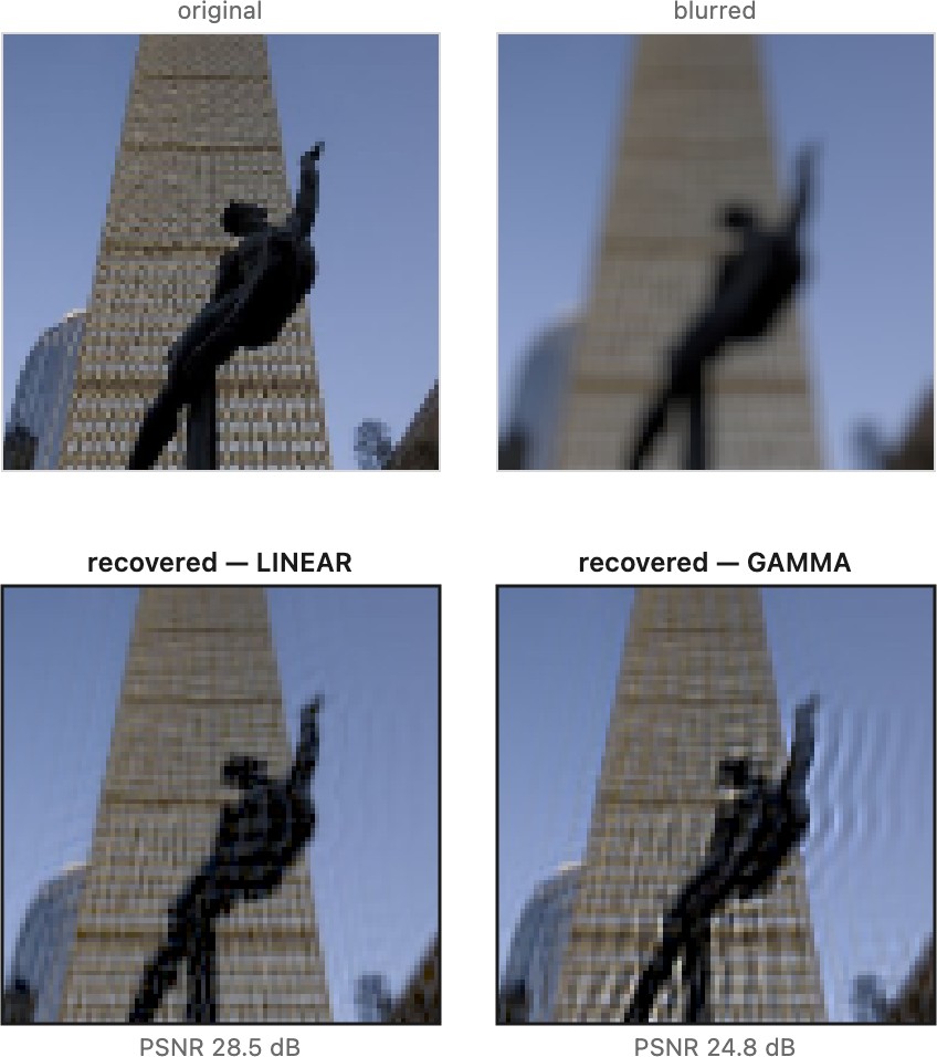
The interactive figure makes the companion lesson (deconvolution belongs in linear light) concrete on a real 2-D image. Blur an image in linear light (the physically correct way, since light adds), then invert the blur two ways. Invert on the linear values and you recover the source. Invert instead on the gamma-encoded values (as you would by feeding 8-bit pixels straight to the solver) and, because gamma and blur do not commute, the result is systematically wrong (halos, lost contrast), a point that returns in Color technology. The figure prints the PSNR of each recovery so the gap is quantified. One caveat, clearest on the default Prudential photo: the gamma error is systematically worse numerically yet not always obvious to the eye: most local neighborhoods of a photo span a narrow range of values where the gamma curve is nearly linear, so the mismatch stays subtle; it is the shadow-dipping grating that makes it plain.
The cure that panel (d) uses is regularization, and it is the most important single idea in this chapter's linear-algebra half. Rather than chase the data exactly (which means chasing the noise) solve a balanced problem:
The first term insists the answer explain the measurement; the second term, $R(\mathbf{x})$, penalizes implausible scenes (ones that are too wiggly, not smooth, not sparse) and the knob $\lambda$ sets how much plausibility is allowed to override data fit. Tikhonov regularization, $R(\mathbf{x})=\lVert\mathbf{x}\rVert^2$ or $\lVert\nabla\mathbf{x}\rVert^2$, simply damps the blow-up on the small singular values and is the classical choice Tikhonov 1963; total variation, $R(\mathbf{x})=\lVert\nabla\mathbf{x}\rVert_1$, penalizes wiggle while sparing edges. This single line (a data term plus a regularizer) is the skeleton of nearly every restoration method in the book, and the broad theory of inverting imaging operators this way is a field of its own Bertero & Boccacci 1998.
It is worth being clear about two kinds of "hard," because they are constantly confused. Some difficulty is merely numerical: the system is enormous and sparse, slow or unstable to solve by brute force. That kind yields to better tools (conjugate gradient, multigrid, FFT-based diagonalization, preconditioning) all of which live in Efficient solvers, and none of which change what is recoverable; they just reach it faster and more stably. But conditioning and rank are properties of $A$ itself. No solver, however clever, recovers a scene direction the null space erased or the noise drowned. The distinction is the whole ethic of this chapter: "hard to compute" is an engineering problem; "impossible to recover" is a fact about the operator and the noise, and the only things that change it are more measurements or a better prior, full stop.
Two complications make the real world harder than this tidy story. First, sometimes you do not know $A$. Blind deblurring, for instance, must estimate the blur kernel and the sharp image at once (solving for the operator and the unknown together) which is dramatically harder and, again, rescued only by priors (now on both the image and the kernel; → 09 Single-image computational photography#Blind deblurring). Second, and more insidiously, sometimes you think you know $A$ but you are wrong: the point-spread function is slightly off, the noise is not quite Gaussian, the optics have drifted. A confident inversion of a subtly mistaken model produces confident artifacts: structure that looks real and is not. Robustness to model error is a real and under-appreciated cost of every method that leans hard on knowing $A$.
Finally, a forward pointer that pays off the whole "conditioning" discussion. Everything above gets dramatically clearer when $A$ is diagonal, because then each direction inverts on its own and you can read off, at a glance, exactly which ones are doomed. For the convolutions that dominate imaging (blur, defocus, motion) the Fourier basis diagonalizes $A$: deblurring becomes per-frequency division, and ill-conditioning becomes simply the frequencies the blur zeroed out. That is the subject of Linearity, Fourier, Aliasing and deblurring, and the classic compromise it produces (the Wiener filter, the noise-aware per-frequency inverse that is exactly a regularized inversion done frequency by frequency) is the bridge from this section's abstract conditioning to a concrete, usable deblurring tool Wiener 1949.
A caution about the word linear, since the whole forward-model picture leans on it. First: linear in what? Our $\mathbf{y}=A\mathbf{x}$ is linear in scene radiance: physical light adds, which is exactly why the model is true of the light arriving at the sensor. It is emphatically not linear in the encoded pixel values you usually have in hand. Ordinary image files are gamma-encoded (and often tone-mapped), a deliberate nonlinear remapping, so feeding 8-bit JPEG numbers straight into a linear solver quietly breaks the model and corrupts the inversion. When linearity matters, and for inversion it matters enormously, work in linear light: undo the gamma first (→ gamma encoding, BASICS). Second, and just as easily muddled: a linear forward model does not make the solution linear. The scene-to-measurement map is linear; the measurement-to-estimate map $\mathbf{y}\mapsto\hat{\mathbf{x}}$ is in general nonlinear, because the regularizer (equivalently, the prior) makes it so: any sparsity penalty, any clamp to valid pixel ranges, any non-Gaussian prior turns recovery into a thoroughly nonlinear function of the data. Linear physics, nonlinear inference.
2.15.2 Priors and the manifold of natural images⧉
The big lesson of the previous section is that our reconstruction problems often simply do not carry enough information to pin down an answer. It is starkest when the operator is underdetermined (fewer equations than unknowns, so a whole null-space of scenes fits the data equally) and again in the purest case of all, denoising ($A=I$): every clean image within the noise level of the measurement is an equally plausible explanation, and the problem as posed is perfectly isotropic: nothing in the measurement or the noise model favors one direction of correction over another. With no further knowledge, there is genuinely nothing we can do.
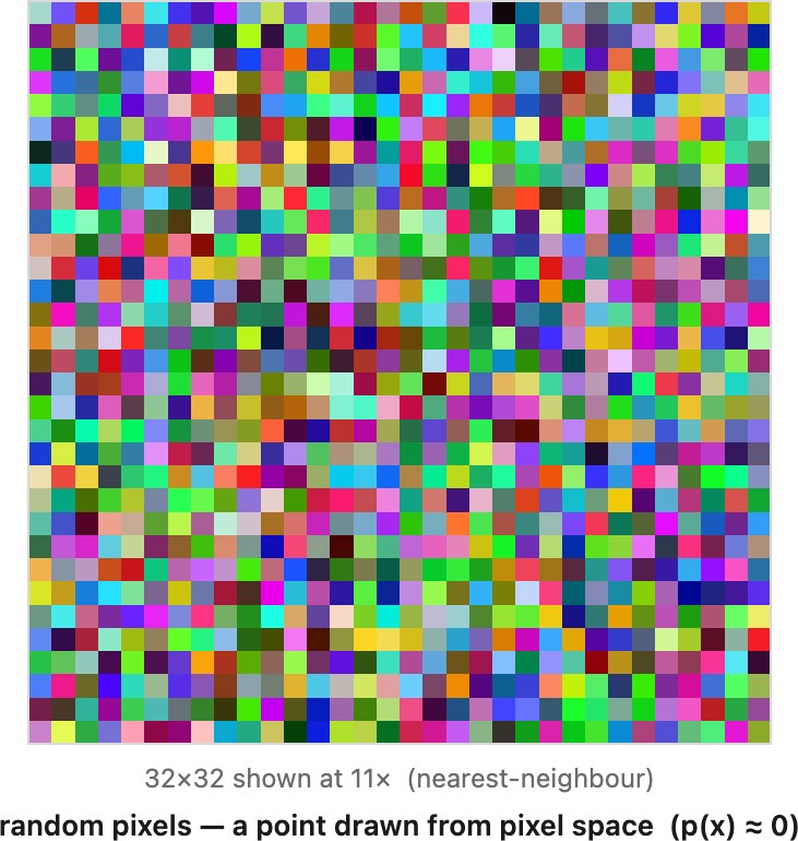
Fortunately, we are almost never after arbitrary images. We want pictures of the world around us, and such images are visually special, sharply distinguished from random arrays of numbers. Press sample random in Figure 2.15.5 and you draw a point uniformly from the space of all images: it is television static, every single time, and no amount of pressing will ever land on a face, a leaf, or even one clean edge. The vast majority of arrays of RGB values look like noise, and look nothing like the photographs anyone actually wants to take.
If we regard an image as a high-dimensional vector in the abstract space of all images (the same space as the linear-algebra section above, one axis per pixel) then the natural images occupy only a tiny, structured region of it. We call that region the manifold of natural images (Figure 2.15.6): the thin, curved sliver where real photographs live and a good prior $p(\mathbf{x})$ is high, adrift in the overwhelming bulk of the space, which is noise and where $p(\mathbf{x})\approx 0$. Do not lean too hard on the word manifold: it is a useful mental picture more than a precise claim, and the locus of natural images very likely does not satisfy the strict properties of a mathematical manifold Kadkhodaie, Guth et al. 2024.
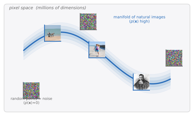
Natural images occupy only a tiny fraction of the space of all arrays of RGB values.
That tiny fraction is exactly the extra knowledge that breaks the deadlock. Take denoising again (Figure 2.15.7). The noise alone leaves a whole cloud of clean images equally consistent with the measurement, and with no prior the best guess (the posterior mean) is simply their average, which works out to the noisy input itself: we have learned nothing. But if we insist the answer be a natural image, most of that cloud is ruled out at a stroke: keep only the candidates on the manifold, and the ambiguity collapses toward the one scene the prior calls a real image.
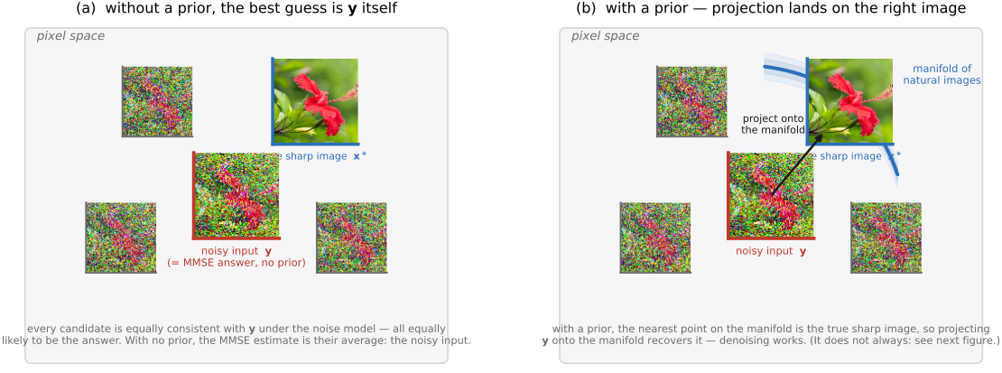
If we can computationally model the manifold of natural images, we can use it to exclude unlikely solutions to inverse problems.
What remains is to make this precise. The next section retells the whole story in the language of probability (likelihood, prior, posterior) which turns "the answer must lie on the manifold" into an exact computation and shows that the prior is the very same object as the regularizer of the linear-algebra view. First, though, a little more about the manifold itself: how using it can go subtly wrong, why the humble denoiser is so central, and what the statistics of real images actually look like.
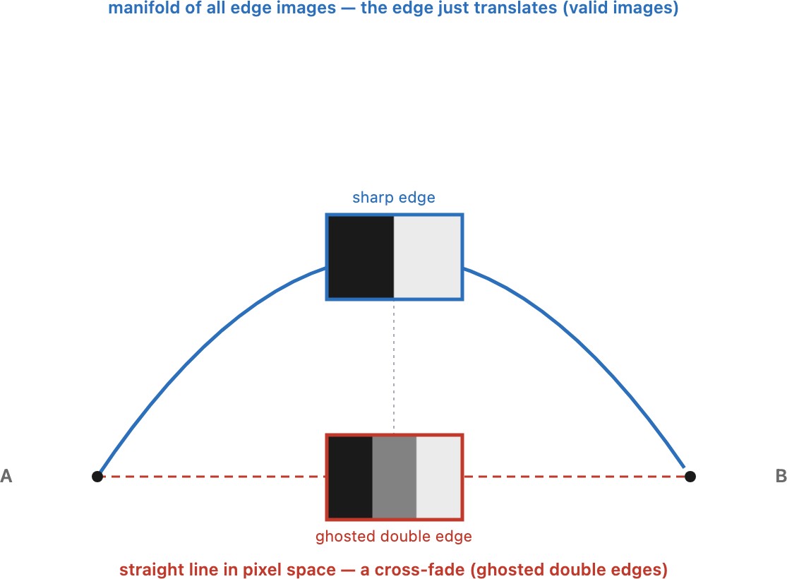
But projecting onto the manifold does not always land on the right image, and that exposes a subtle trap in how one uses a prior (Figure 2.15.8). When the plausible true images sit on different parts of a curved manifold, the "safe" posterior mean averages them, and the average cuts a chord across the bend and lands off the manifold, as a blurry, washed-out image. This is the precise sense in which the average can be dull: the estimate that is optimal in squared error need not be a valid image at all. It is why a perfectly-trained MMSE denoiser still over-smooths, and why the sampling of a generative prior (committing to one sharp point on the manifold) can look better than the safe average.
This special status is worth dwelling on, because it explains a great deal of modern imaging. Denoising is the inverse problem stripped to nothing but the prior ($A=I$): its entire job is to take an ambiguous point and snap it onto the manifold. That perfect symmetry and ambiguity are exactly what make the denoiser a universal building block. Since a denoiser is operationally a projection toward the manifold, any good denoiser doubles as a prior you can drop into other inverse problems (use it as the regularizer in deblurring, super-resolution, or inpainting) which is the plug-and-play / RED idea developed in Image priors. And it is the seed of generative AI: a diffusion model is trained as a denoiser across many noise levels, and sampling from it (repeatedly denoising starting from pure noise) is nothing but walking onto the manifold one small step at a time. So the humblest inverse problem turns out to be the most central: the ability to snap to the manifold is why one operation became, at once, a universal family of priors and the engine of modern image generation (Image priors; generative diffusion).
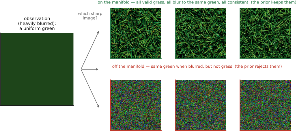
Even a perfect manifold does not save us entirely. It shrinks the set of possible answers, but many candidates can remain on the manifold, all equally consistent with the measurement. Consider a photo of a grass field blurred so heavily that it is a uniform green (Figure 2.15.9). That observation carries no information at all about where the individual blades lie: a great many different natural images of grass, blurred that much, would produce the very same uniform green, and the prior has no way to choose among them. What it can do is rule out the noise images, which lie off the manifold. So the prior narrows the field but still leaves a whole family of plausible answers. How much the manifold actually buys us, made quantitative, is what Levin and colleagues measured for denoising [@levin-nadler-2011; @levin-etal-2012-patch]; we point there for the numbers.
We are not flying blind about the manifold's shape; decades of work have measured its regularities, and they are exactly what priors exploit. Natural images have $1/f$ amplitude spectra, a scale-invariance that says structure exists at every scale [@field-1987; @ruderman-bialek-1994]. Their gradient and wavelet statistics are heavy-tailed: mostly near-zero (smooth regions) with rare large values (edges), which is the precise meaning of sparsity and the basis of sparse-coding models of early vision Olshausen & Field 1996. They have strong local correlation. There is even a strikingly simple generative model that produces all of this at once, the dead-leaves model: opaque shapes of random size and brightness dropped one atop another, with a power-law distribution of sizes, so that occlusion alone reproduces the $1/f$ spectrum, the scale-invariance, and the heavy-tailed edge statistics (Matheron's random-set geometry; Lee, Mumford & Huang 2001 Lee, Mumford & Huang 2001 (dead leaves); Ruderman 1997 Ruderman 1997). It is the classic bridge from measuring image statistics to modeling them, and the hand-built ancestor of today's learned generative priors (diffusion). Each of these regularities is, quite literally, what a classical regularizer encodes (total variation bets on sparse gradients, wavelet priors on sparse coefficients) and the whole program of reading images off their statistics is a well-developed science [@simoncelli-olshausen-2001; @hyvarinen-etal-2009].
The arc of the field is a march from hand-written priors to learned ones. The early priors (smoothness, total variation, a handful of wavelet coefficients) are easy to write down and coarse: they capture a little of the manifold's shape and miss most of it. Modern priors are learned from millions of images and capture it astonishingly well. The strongest learned prior we have is, in fact, a generative model: a diffusion model is, at heart, precisely a learned model of $p(\mathbf{x})$ (of the natural-image manifold itself) and it is the subject of the final chapter of 05 Computational tools, Generative AI and diffusion. That is the teaser; the machinery that turns any such prior into a restoration engine (the realization that any denoiser secretly is a prior, and that diffusion is iterated denoising) is Image priors, where that thread is picked up.
There is a useful way to name what is shifting underneath that arc. Every method bakes knowledge about images in one of three forms: an explicit prior (a penalty you write down: smoothness, total variation, sparsity); an inductive bias (assumptions built into the machinery rather than stated: a wavelet basis, a convolutional network's translation-equivariance and locality, the architecture itself); and data (regularities absorbed by fitting millions of examples). The history of image priors is a steady transfer of weight from the first two to the third, and that transfer is a local instance of Rich Sutton's "bitter lesson" Sutton 2019: across AI, general methods that simply scale with computation and data have repeatedly overtaken systems built on hand-engineered human knowledge. It is bitter because the clever, interpretable priors that researchers labor over keep getting bulldozed by a bigger model that has merely seen more images, but the pattern has held. For our problem it means a learned model that has seen the manifold beats any penalty we can write down to describe it. The clear-eyed caveat is that the bitter lesson is about what wins at scale, not about what is understandable or data-efficient: hand-built priors and architectural inductive biases remain the right tool when data is scarce, when guarantees matter, or when you must know why an answer came out, which is much of scientific and medical imaging, and anywhere outside the data-rich consumer-photo regime.
2.15.3 Probability: the Bayesian view⧉
Now the same problem, retold in the language of probability, and this is the more fundamental telling. We do not really want an $\mathbf{x}$ that happens to fit; we want the most probable scene given the measurement, fusing two sources of belief: what we just observed, and what we expected beforehand. Bayes' rule states the fusion exactly:
Read this way, every imaging inverse problem has exactly three ingredients, and it pays to hold them apart: a forward model (the operator $A$, how a scene turns into a measurement), a noise model (the statistics of $\mathbf{n}$, how that measurement is corrupted), and a prior (which scenes are plausible before we look at all). The first two together are the likelihood $p(\mathbf{y}\mid\mathbf{x})$; the third is $p(\mathbf{x})$. Naming the three is more than tidiness. It is what lets you change one without disturbing the others: a new camera changes only the forward model, a noisier sensor only the noise model, a better image model only the prior.
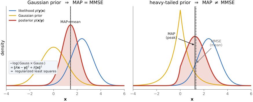
The likelihood $p(\mathbf{y}\mid\mathbf{x})$ is nothing other than the forward model plus the noise model: it scores how well a candidate scene explains the data. For $\mathbf{y}=A\mathbf{x}+\mathbf{n}$ with Gaussian noise of variance $\sigma^2$, it is $p(\mathbf{y}\mid\mathbf{x})\propto\exp\!\big(-\lVert A\mathbf{x}-\mathbf{y}\rVert^2/2\sigma^2\big)$, which is the data-fit term from the previous section, wearing a probability hat. The prior $p(\mathbf{x})$ is everything we know before looking at this particular measurement: that natural images are smooth in places and edgy in others, that they are emphatically not random noise. It is the principled relative of the regularizer, related by $R(\mathbf{x})\leftrightarrow-\log p(\mathbf{x})$. Where regularization felt like a numerical trick ("add a penalty so the answer behaves"), the prior is a statement about the world, one you can argue about, measure on real photographs, and improve. That is why it is philosophically the more grounded notion, and practically the more general one: a prior need not be Gaussian; it can be heavy-tailed, multimodal, or learned from data (Figure 2.15.10).
2.15.4 Optimization, inference, loss⧉
We now have everything the problem is made of: a forward model (linear or not), a noise model, and a prior; together, a posterior $p(\mathbf{x}\mid\mathbf{y})$ that scores every possible scene. But a posterior is a whole distribution over answers, and a user wants one image. So the question that every restoration method answers, whether or not it admits it, is: given the distribution of plausible solutions, what single answer do we return? There is a small menu, and the choice is a real one: it is the moment inference, optimization, and the notion of "loss" all enter.
Pick the most probable one: MAP. The simplest answer is the peak of the posterior, the single most probable scene: the maximum-a-posteriori (MAP) estimate. Take the negative logarithm of the posterior and minimize:
This is where inference becomes optimization, and the coincidence that makes the two halves of this chapter one picture. If the prior is Gaussian, $-\log p(\mathbf{x})$ is a quadratic, and this is exactly the regularized least squares of the linear-algebra view, with $\lambda\propto\sigma^2$. So regularization is MAP under a Gaussian prior: the very same minimization, told two ways. The $-\log$ is the whole trick: it turns a product of probabilities into a sum of penalties, a data term and a prior / regularization term. Whenever you see a regularizer, read it as the negative log of a prior, and ask the plain question behind it: what distribution of scenes does this penalty actually assume?
Minimize an aggregate distance to the plausible solutions, and which distance? MAP returns the single likeliest scene, but that is not the only thing one might want. Instead of the peak, we can return the answer that is, on average, closest to the true scene, closest in some chosen notion of distance. Minimize the expected squared error and you get the MMSE estimate, the posterior mean, the average over all plausible scenes (and, a fact we lean on hard later, exactly what an optimal denoiser returns, the hinge to Image priors and Tweedie's formula). But "closest" begs the question which distance? Squared pixel error is merely the convenient choice (its derivative is linear, so it is easy to optimize) not the right one. Two images a person would call identical can be far apart in pixel $L_2$, and two that $L_2$ calls close can look obviously different. The distance you minimize is a loss, and choosing it is choosing what you are willing to be wrong about: a numerical loss ($L_2$, $L_1$) is tractable but perceptually naive; a perceptual loss (SSIM, LPIPS, a deep feature distance) is closer to what the eye scores but harder to optimize and easier to game (→ Image metrics; perceptual and adversarial losses in Deep learning). The loss defines what the method treats as a good reconstruction.
Sample them: posterior sampling. A third answer gives up on a single best estimate altogether: draw a sample from the posterior, commit to one plausible scene, sharp and self-consistent, rather than a summary of all of them. This is what generative restoration does (diffusion posterior sampling and its kin), and it is often the most natural-looking answer even when it is neither the most probable nor the closest-on-average one, because a sample lands on the image manifold, where an average falls off it.
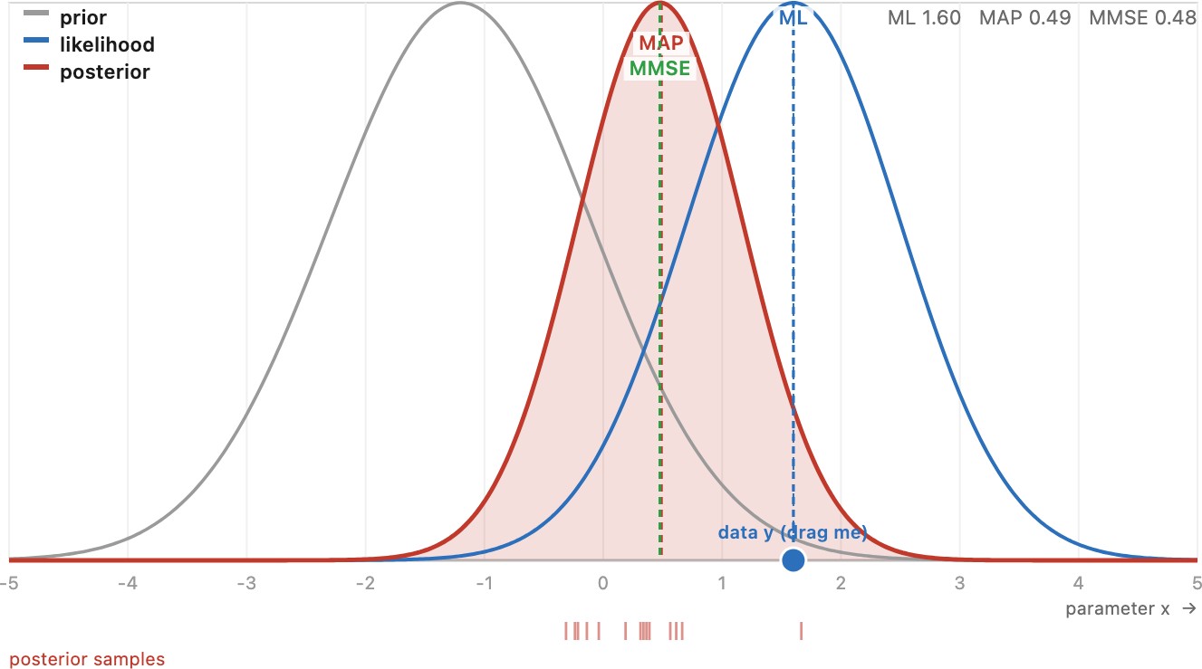
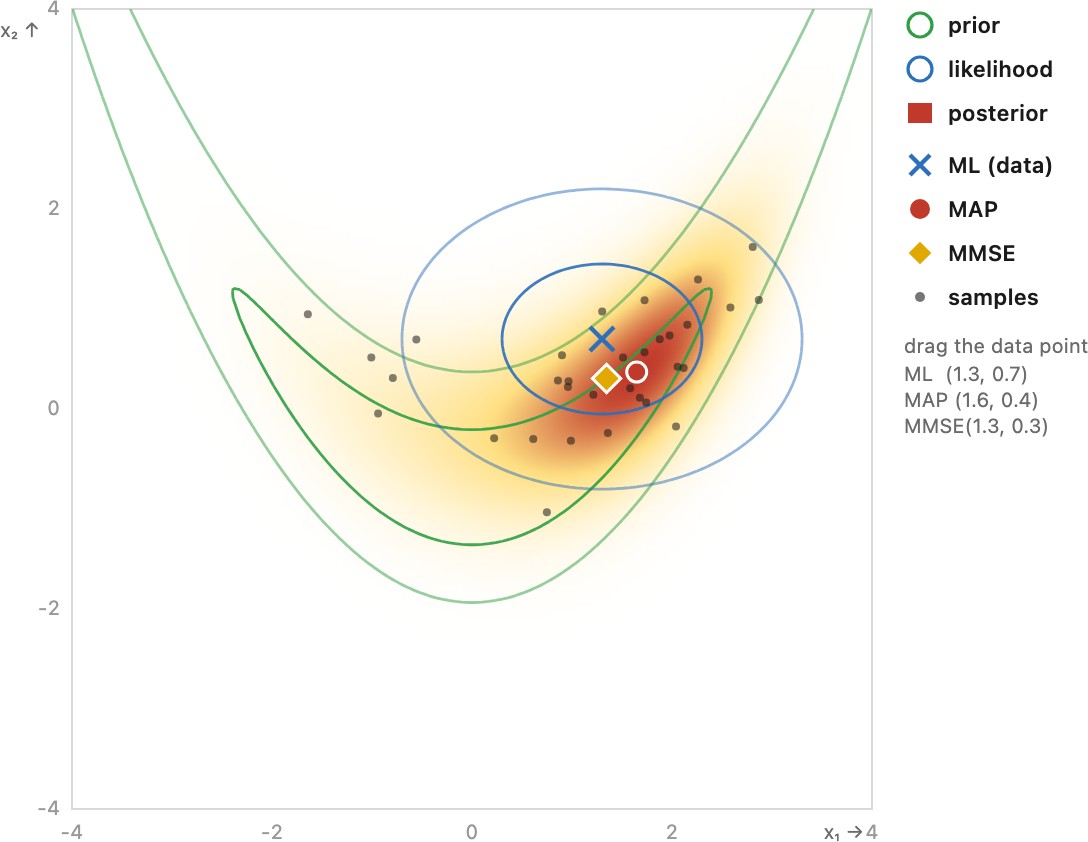
These three are not interchangeable. For a Gaussian posterior the peak and the mean coincide and the distinction is academic. But natural-image priors are heavy-tailed, their posteriors skewed or multimodal, and then MAP, MMSE, and a posterior sample can sit far apart: the MAP perched on a sharp narrow peak the mean is nowhere near, a sample off on the manifold where neither sits (Figure 2.15.10). Which one is "right" depends entirely on what you are paying for Kay, Estimation Theory. What all three share is the prior: by either name (regularizer or prior, loss or likelihood) the lesson is the book's L5.4, for an ill-posed problem the prior is not optional. It is the only thing standing between you and the noise.
Two practical observations close the Bayesian picture. The first is a piece of luck peculiar to photography: data is cheap. Building or learning a good prior $p(\mathbf{x})$ wants a great many example images, and photography has them by the billion, unlike, say, black-hole imaging, where the Event Horizon Telescope must reconstruct a picture from a single, precious, radically incomplete measurement with essentially no ground truth to lean on. By comparison we are spoiled for data. The caveat is that fully ground-truthed data is rarer than it first appears: even for demosaicking, the "true" full-color image hiding behind a Bayer mosaic is not something a camera can simply hand you, so the data we train and validate on is often itself a stand-in for a ground truth we never quite had.
The second observation is that the prior is there whether you name it or not. A bilateral filter, an edge-aware demosaicking rule, a hand-tuned denoiser, an end-to-end neural network. None of these mentions a prior, yet each embeds one: a bet about what natural images look like, welded into the method's machinery. The bet gets made regardless; the only question is whether you made it on purpose. This is the quiet virtue of the Bayesian formulation: it cleanly disentangles the three ingredients (forward model, noise, prior) from the inference method that fuses them, which is more modular and theoretically cleaner (sharpen the prior, and every task that borrows it improves at once; → Image priors). That clean separation is not always achievable, and insisting on it can leave performance on the table: a tightly coupled end-to-end method that refuses to factor may simply work better. But knowing where your prior lives, even when it is implicit, is much of the difference between engineering and luck. So the natural next question is the one the rest of the chapter answers: what is that prior?
2.15.5 When you can design the operator — and a teaser of information theory⧉
So far we have taken the operator $A$ as a given (handed to us by the optics) and asked only how to invert it. But a recurring theme of computational photography is that $A$ is often ours to choose. A coded aperture swaps the clear lens stop for a designed mask; a light-field camera inserts a microlens array; a coded exposure flutters the shutter; an end-to-end-optimized lens is allowed to shape its own point-spread function. The moment you have that freedom the problem changes character: it is no longer "invert this $A$," but "design the $A$ (together with its reconstruction) that makes the whole pipeline work best." Acquisition and recovery become a single, jointly optimized system, and the goal is to pick the operator whose measurements carry the most recoverable information about the scene, not merely the prettiest raw image. (Coded imaging redesigns $A$ to be better-conditioned; light fields and multi-shot capture make $A$ taller, both are this same move, and both get their own parts: 16 Computational optics and coded imaging, 14 Light fields and plenoptic cameras.)
That raises a question the inverse-problem view cannot answer on its own: given the freedom to choose $A$, which choice is best? The tool for reasoning about it is information theory, which gets its own chapter in Computational tools. There an imaging system is read as a communication channel (a noisy, band-limited pipe from scene to sensor) with an information capacity ($C=\int\log_2(1+\mathrm{SNR}(f))\,df$ across spatial frequencies) that measures how many bits of scene a given $A$ can actually deliver. That capacity is exactly the yardstick for designing $A$: choose the operator that maximizes the information the measurement carries, then reconstruct. One flag on its reach, though, worth planting now: information theory is powerful on the measurement-and-transport side of imaging, how efficiently a system captures, stores, and moves image data (the channel, compression, detector efficiency), and largely silent on the perceptual and aesthetic side; it has nothing to say about what makes a photograph look good. It governs precisely the part of imaging this chapter is about (recoverable information) and stops where taste begins. A concrete, long-shipped instance worth flagging is gamma encoding in television: spending a limited, noisy set of transmission levels where the eye can tell them apart (fine steps in the shadows, coarse in the highlights) is applied information theory decades before it wore the name. (We unpack its noise rationale where encoding is developed, in Color technology.)
2.15.6 Recap: what makes imaging hard, and where it's going optional⧉
The chapter reduces to a small set of recurring ideas. The fundamental equation $\mathbf{y}=A\mathbf{x}+\mathbf{n}$ is hard to invert for two reasons, and only two: the noise $\mathbf{n}$ corrupts the data, and the operator $A$ loses information, by being rectangular (a null space the data cannot fill) or non-invertible / ill-conditioned (singular values at or near zero, so inversion amplifies noise without bound). Because information is genuinely gone, recovery requires extra knowledge (a regularizer, or equivalently a prior) and that is not a workaround but a logical necessity.
One assumption ran underneath all of it, and it is worth flagging before we move on: the forward model here is linear (the data is a linear map $A$ of the unknown plus noise) which is what let us bring the whole machinery of linear algebra, Fourier analysis, and least squares to bear. That covers a huge swath of computational photography (blur, downsampling, missing pixels, tomographic-style mixing), but it is not universal. Some problems are genuinely non-linear in the unknowns, because the unknowns multiply each other rather than combining additively: when the scene depth is unknown the warp that relates two views depends on depth times motion, and in transparency / matting the observed color is $\alpha F+(1-\alpha)B$ (foreground times its own opacity) so the unknowns are coupled multiplicatively. Those problems inherit all the ill-posedness of this chapter and add non-linearity on top, which is why they need their own treatment (the matting equation is taken up in Compositing, segmentation and matting).
The cleanest way to feel this is to strip the problem to its core. Set $A=I$ (no blur, no sub-sampling, just $\mathbf{y}=\mathbf{x}+\mathbf{n}$) and you have denoising, the quintessential inverse problem. It sits at one extreme of the whole space of inverse problems: the operator is as benign as it can possibly be (the identity, with literally nothing to invert) and yet recovery is still impossible without help. That is the cleanest possible proof that the difficulty was never only about undoing a hard operator: even when there is no operator to fight, the noise alone leaves the problem ill-posed, and only extra knowledge resolves it. (The other extreme is where $A$ is the villain, rectangular or ill-conditioned, and the two failure modes blur together in between.) Notice what happens to the data term: with $A=I$ it does nothing to distinguish candidates, because every $\mathbf{x}$ explains the data about equally once you grant the noise. The prior therefore does 100% of the work. Without any knowledge of what natural images look like, you cannot denoise at all: there is no principled way to tell signal from noise; with that knowledge, you can. Denoising is the inverse problem reduced to its essence (the operator stepped out of the way so that only the prior remains) which is exactly why "any good denoiser is a universal prior" became the organizing idea of modern restoration (Image priors).
So, one last time, the two perspectives reconcile: linear-algebra regularization and Bayesian prior are the same method whenever the noise is Gaussian, the observation is linear, and you take $-\log$ and maximize: regularized least squares is MAP under a Gaussian prior. The Bayesian view remains the more general of the two (non-Gaussian priors, the MAP-versus-MMSE choice, learned $p(\mathbf{x})$), and it has the virtue of telling you where the regularizer came from in the first place.
That reconciliation also frames the big trend worth ending on. Historically, the two halves of $\mathbf{y}=A\mathbf{x}+\mathbf{n}$ got uneven attention. We became extraordinarily good at the measurement side (precise forward models $A$, exact least-squares and Fourier and Wiener inversion, the whole conditioning analysis of this chapter) while priors stayed coarse: smoothness, total variation, a few wavelet coefficients, the hand-written regularizers. Generative AI has flipped the balance. Diffusion models give us astonishing priors (a near-perfect grip on the natural-image manifold) but it has proven hard to keep their output faithful to the measurement: the data-fit $\lVert A\hat{\mathbf{x}}-\mathbf{y}\rVert$ can drift, and the model "hallucinates" detail that is plausible under the prior but wrong given the data. The live research frontier is therefore to honor both at once (the measurement and the learned prior) which is what diffusion posterior sampling, denoising diffusion restoration, and plug-and-play methods with learned denoisers are all reaching for [@kadkhodaie-simoncelli-2021; @chung-etal-2023-dps; @kawar-etal-2022-ddrm].
And that is the hand-off to the rest of the book. Every later restoration chapter is a special case of this one: choose the operator $A$, choose a prior on $\mathbf{x}$, and balance data fit against it. The solvers that carry it out are Linear inverse problems and regression; the Fourier picture that makes the conditioning legible is Linearity, Fourier, Aliasing and deblurring; and the priors, from hand-built penalties through learned denoisers to diffusion, are Image priors and Generative AI and diffusion. We opened by writing the camera's forward model backward; the rest of the book is learning to solve it.
2.15.7 Harder inverse problems: factorization⧉
Everything above assumed the forward model is linear: a known operator $A$ acting on one unknown. A whole second family of problems drops that, and it is worth naming before we leave the chapter, because it recurs constantly. In these the measurement is a product of two unknowns, and we must recover both factors from their product alone.
The canonical version is pure arithmetic. Hand someone the number 12 and ask which two numbers were multiplied to make it. The answer is radically underdetermined: $3\times4$, $2\times6$, $1\times12$, $2.4\times5$ all fit, and nothing in the product alone prefers one. Only extra knowledge (a prior on what each factor is allowed to be) breaks the tie. That is the same logical move as regularization above, now doing even heavier lifting.
Factorization problems seek to decompose a number, or an image, into a product of two unknown pieces (scalars, or whole matrices) given only the product. This is fundamentally ill-posed: many factor pairs multiply to the same result, and there is always the degenerate "put everything in one factor, leave the other the identity" split. Only a prior on each factor breaks the tie. In the fully general case it is our linear problem $\mathbf{y}=A\mathbf{x}+\mathbf{n}$, except we must now solve for the operator $A$ as well as the unknown $\mathbf{x}$. Examples include white balance, intrinsic images, matting, and blind deblurring.
In the fully general case, factorization is our familiar linear problem $\mathbf{y}=A\mathbf{x}+\mathbf{n}$ with the ground shifted beneath it: now $A$ is unknown too, and we must recover the operator and the scene it acted on from their product alone. That extra unknown is what tips these problems from merely ill-conditioned to genuinely ambiguous.
A striking number of imaging problems are exactly this shape:
- White balance: the raw sensor value is (to first order) the illuminant times the surface reflectance: $\text{observed}=\text{light}\times\text{material}$. From the product we must separate what color the light was from what color the object is. How hard the factorization is depends on how much we let the light vary. Global white balance assumes one illuminant for the whole frame, so a single triplet of coefficients (three numbers) explains every pixel: the factorization is heavily over-constrained and usually easy. Local (spatially varying) white balance lets the light change across the scene, so each pixel becomes its own independent product of two color triplets, the local light times the local material. That is far more ambiguous, and it takes a strong prior on how illumination varies to pin it down (Figure 2.15.13) [@hsu-etal-2008; @boyadzhiev-etal-2012].
- Intrinsic images: an image is shading times reflectance (albedo), $I=S\times R$: the geometry-and-illumination term times the material term. Split them and you can relight, recolor, or lift shadows.
- Matting: a composited pixel is $\alpha F+(1-\alpha)B$: foreground color, background color, and opacity $\alpha$, coupled multiplicatively into one observed color (the equation of Compositing, segmentation and matting).
- Blind deblurring: the blurry photo is the sharp image multiplied by an unknown blur matrix (blurring is a linear operator, so the observation is the product of that operator with the image) and we know neither the image nor the blur (Blind deblurring).
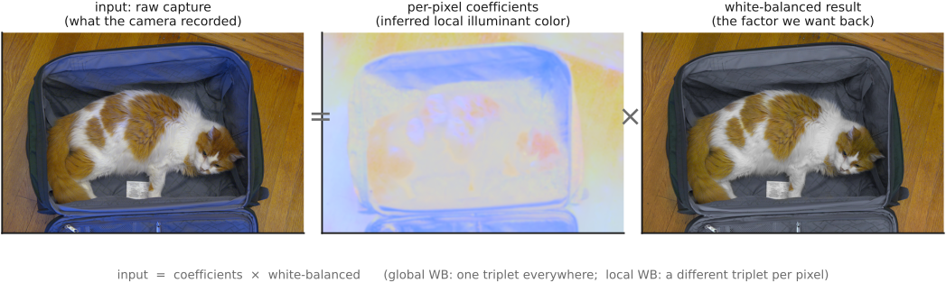
These factorization (or blind, or separation) problems share two features. First, they are even more ill-posed than a linear inverse problem, because there is always a trivial degenerate split: dump everything into one factor and leave the other the identity (the "$1\times12$" answer, which for blind deblurring is precisely the "no blur, the image is already sharp" trap). Only a prior on each factor (illuminants are few and smooth, reflectances piecewise-constant, natural images sparse-gradiented, mattes nearly binary) makes the split unique. Second, the forward model is no longer linear, but it is usually _multilinear_: linear in each factor separately while the others are held fixed ($\alpha F$ is linear in $F$ for fixed $\alpha$, and linear in $\alpha$ for fixed $F$; $S\times R$ likewise). That structure is exactly what keeps them tractable: it invites alternating schemes (freeze one factor, solve the other as an ordinary linear problem, alternate), which is why so many of these methods read as coordinate descent. Seen this way, white balance, intrinsic images, matting, and blind deblurring are the same structural problem in four different applications: recover the factors from their product, and use a prior to choose among the many that fit.
Recap: big lessons of this chapter
Inverting $\mathbf{y}=A\mathbf{x}+\mathbf{n}$ is hard for exactly two reasons: the operator and the noise. The noise $\mathbf{n}$ corrupts every measurement, so even a perfectly invertible $A$ hands back a corrupted answer. And the operator $A$ throws information away: it can be rectangular (fewer measurements than unknowns, as in the Bayer mosaic, which records only one color channel per pixel) or ill-conditioned: technically invertible but crushing some directions of the scene almost to zero, as in the blur from camera shake, so undoing it divides by almost nothing and detonates the noise. Two further twists make it worse: sometimes $A$ is itself unknown and must be estimated alongside the scene (blind deblurring), and even when it is nominally known, modeling $A$ precisely is hard: a subtly wrong operator yields confident artifacts. Everything downstream in this chapter is the fight against these.
Natural images occupy only a tiny fraction of the space of all arrays of RGB values.
If we can computationally model the manifold of natural images, we can use it to exclude unlikely solutions to inverse problems.
Factorization problems seek to decompose a number, or an image, into a product of two unknown pieces (scalars, or whole matrices) given only the product. This is fundamentally ill-posed: many factor pairs multiply to the same result, and there is always the degenerate "put everything in one factor, leave the other the identity" split. Only a prior on each factor breaks the tie. In the fully general case it is our linear problem $\mathbf{y}=A\mathbf{x}+\mathbf{n}$, except we must now solve for the operator $A$ as well as the unknown $\mathbf{x}$. Examples include white balance, intrinsic images, matting, and blind deblurring.