2.14 Imaging as a linear system🔗⧉

The image-measurements chapter ended with a single pixel: its value is an integral of the light against a sampling kernel. That is true, but it is a statement about one number. A photograph is millions of numbers, and the whole point of computational photography is to reason about the camera that produced them — to ask not just "what did this pixel measure?" but "what did this camera, as a whole, do to the scene?" This chapter gives that question a single, compact answer.

Every imaging system can be written as a linear map. Discretize the scene into a list of numbers — a vector $\mathbf{x}$ — and discretize the image the same way into a vector $\mathbf{y}$, and the camera is a matrix $A$:

In words: the measured image is the matrix $A$ times the scene, plus measurement noise $\mathbf{n}$. This is nothing more than the image-measurements chapter's "a pixel is an integral," repeated for every pixel and with all the weights kept. Each pixel value was a weighted sum of scene radiances; collect the weights for pixel $i$ into the $i$-th row of $A$, and the matrix–vector product reproduces every one of those integrals at once. The content of this chapter is the realization that follows: which weights you put in $A$ is the imaging system. A pinhole, a lens, a coded aperture, a stereo pair — they differ only in their matrix.

This is the part's big lessons made concrete. We said image formation is selecting and combining rays: a pinhole selects a single ray for each pixel, a lens combines a whole cone of them. The matrix $A$ is exactly that selection-and-combination, written down. A row that is zero everywhere except one entry selects one scene element; a row full of small weights combines many. Read a camera's matrix and you have read what the camera does to light.

To keep $A$ small enough to look at, we work in flatland, a two-dimensional world with a one-dimensional scene and a one-dimensional sensor, and we discretize both, so that $A$ is a modest matrix we can draw as a picture (Figure 2.14.1). Everything generalizes to the real 2-D-scene, 2-D-sensor case; the matrices just get larger (a 2-D image flattened into a long vector, $A$ correspondingly huge), and they are too big to draw but conceptually identical. Flatland loses nothing essential and gains a matrix we can see.

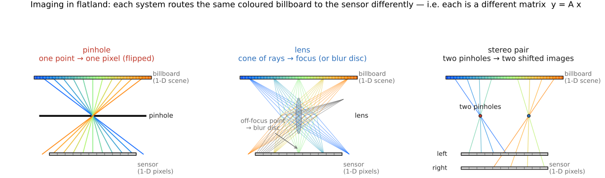
How we feed $A$ depends on how we choose to write down "the scene." There are two standard parameterizations, and the difference between them is the spine of this chapter. The first treats the scene as a flat billboard at a fixed depth — a single row of colored points. It is the obvious choice, it makes the matrices concrete, and it has one sharp limitation we will hit head-on. The second treats the scene as ray space — the set of all rays, the light field — and it is the parameterization that removes the limitation. We take them in turn.

2.14.1 Linear systems from a billboard to an image🔗⧉

Start with the simplest possible scene: a flat billboard standing at some chosen depth, facing the camera, painted with a 1-D pattern of color. Discretize it into a row of points, stack their values into $\mathbf{x}$, and ask what matrix each flatland camera applies. Because the billboard is flat and at a known depth, each system's $A$ is a small matrix we can render as a heat-map — bright where the weight is large, dark where it is zero — and the shape of that heat-map is the character of the camera (Figure 2.14.2).

• Pinhole. Each sensor pixel sees, through the tiny hole, exactly one point of the billboard. The matrix is essentially a permutation — one bright entry per row, zero elsewhere — a re-indexing of the scene onto the sensor. It is as sharp as imaging gets, and it throws away nearly all the light (every ray that does not pass through the hole is discarded). Sharp because each row selects; dim because it selects only one ray.
• Pinspeck. Block the rest of the scene and leave a single small occluder instead of a single small hole, and you get the pinhole's photographic complement — an "anti-pinhole." Its matrix is the all-ones matrix minus the pinhole's pattern: each pixel sums all but one of the scene's contributions. This is the principle behind accidental and occluder-based cameras, where an everyday object's shadow inadvertently encodes an image of the room.
• Lens. Each pixel now integrates a range of billboard points — the cone of rays the aperture admits — so the matrix is a banded blur matrix: a diagonal smeared into a band. On the focal plane the band collapses to the diagonal (sharp, $A\approx$ identity) and off it the band widens (the defocus disc, the circle of confusion from the lens chapter). The lens combines where the pinhole selects — far more light, at the cost of a single plane of focus.
• Corner camera. Let an occluding edge — the corner of a wall — cut across the scene. As you scan past the edge, each successive pixel sees one more sliver of the hidden region than the last, so the measurement is a cumulative sum of the scene and $A$ is essentially lower-triangular. The payoff is that differentiating the measurement undoes the cumulative sum and recovers the scene's angular structure — which is how the faint penumbra at a corner can be read as an image of what is around it.
• Stereo pair. Two pinholes side by side give two images; stack them and $A$ simply gets taller — more rows, two viewpoints of the same scene. The shift of a point between the two halves (its disparity) inverts to depth, which is the whole of stereo (Multiple view geometry). The lesson worth flagging now: more rows means more measurements, and more measurements can carry extra information — here, depth.
• Coded aperture. Replace the lens's clear aperture with a patterned mask. Now $A$ is a coded blur — still a banded matrix, but with a deliberately chosen pattern of weights rather than a smooth disc. The point of the design is to make that blur invertible: a clear disc blurs away certain spatial frequencies irretrievably, whereas a well-chosen code keeps all of them, so the blur can be undone and (as a bonus) the scene's depth read off from which code best deblurs it. We are only naming it here; the design and the deconvolution are the subject of coded aperture.

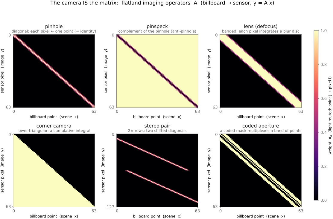
Six cameras, six matrices, one picture each — and that gallery is genuinely the content of half this book in miniature: design the matrix, and you have designed the camera.

This billboard parameterization is tied to a single depth. The matrix $A$ for the lens was a band whose width came from how far the billboard sat from the focal plane; the matrix for the stereo pair encoded a disparity that came from the billboard's distance. Move the billboard nearer or farther and every one of these matrices changes — the lens band widens, the stereo shift grows. A billboard matrix describes the imaging of one flat scene at one depth, and a real scene has many depths at once. We need a way to write down the scene that does not bake in a depth. That is exactly what the light field does.

2.14.2 Linear systems from ray space (light fields) to an image🔗⧉

The fix is to stop describing the scene as a surface and start describing it as rays. Instead of "the color of the billboard at position $u$," take as the unknown "the radiance of the ray arriving at the camera from direction so-and-so, through aperture position so-and-so." The full set of those rays is ray space — the light field (Part 13) — and stacking all of it into $\mathbf{x}$ gives a parameterization that knows nothing about depth: depth is no longer a property of the operator; it is structure inside $\mathbf{x}$ (a depth edge is a particular pattern of which rays carry which color).

Once the scene is ray space, the imaging system becomes a fixed linear projection of that ray space down to the image — and crucially, the projection no longer depends on scene depth. One matrix describes the camera for every scene, because the scene's depth has moved out of $A$ and into $\mathbf{x}$. The same cameras from the billboard gallery reappear, now as different ways of slicing the one light field (Figure 2.14.3):

• a pinhole keeps only a thin slice of ray space — the rays through one point;
• a lens integrates ray space along a sheared line — it sums all the rays in the aperture that converge to one image point, and the shear of that line is the focus setting (refocusing is re-shearing);
• a stereo pair or light-field camera keeps more of ray space — more rows — which is exactly why it can recover depth and refocus;
• a coded aperture keeps a coded projection of the aperture's rays;
• wavefront coding and a focus sweep are yet other linear slices.

Every camera is a different projection of the same underlying light field. That single picture — drawn here after Levin, Freeman and Durand — ties the whole "cameras differ by how they slice the light field" theme together, and it is the reason the operator view is worth installing now.

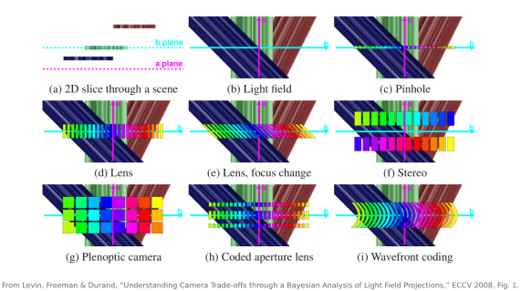
This ray-space view is the natural home of the linear-system framing — Torralba, Isola and Freeman develop the camera as a linear system in exactly these terms Torralba, Isola & Freeman, Foundations of Computer Vision, and the Bayesian trade-off analysis that this figure comes from compares cameras precisely by how their light-field projections behave Levin, Freeman & Durand 2008. The idea to carry out of this section is the thesis of much of the rest of the book: a great deal of computational photography and computational optics is the search for new linear imaging systems $A$ — paired with the reconstruction method that inverts each one — that pull better images and extra information, notably depth, out of the light.

2.14.3 Space–time: imaging across time🔗⧉

So far $\mathbf{x}$ has held a static scene. Add time as another axis of $\mathbf{x}$, a moving scene captured over an exposure, and the picture is unchanged: it is still $\mathbf{y}=A\mathbf{x}$, now over space and time. The previous chapter already noted that the exposure is an integral over time; here that integral is just more rows and columns of $A$. A moving point smears along its trajectory, and motion blur is a linear operator whose kernel is the path the point traced during the exposure.

The trouble with ordinary motion blur is that this operator depends on the scene: a fast object blurs differently from a slow one, and you cannot deconvolve away a blur whose kernel you do not know and which differs across the frame. Motion-invariant photography turns this into an engineering opportunity. Sweep the camera along a carefully chosen parabolic trajectory during the exposure, and the blur point-spread function comes out the same for every object speed — the parabolic sweep is designed so that whatever an object's velocity, it spends matched time at matched positions, yielding one velocity-independent blur (Figure 2.14.4). A single deconvolution then sharpens objects moving at any speed.

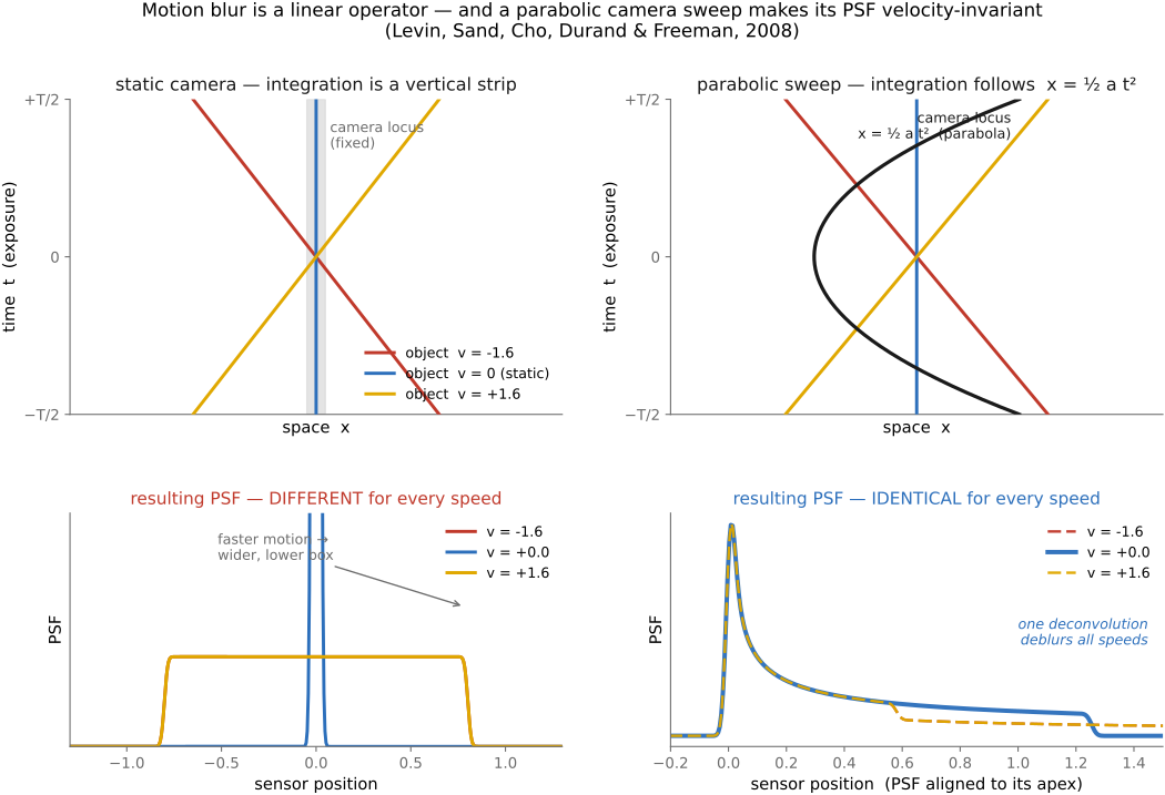
The move is the same one coded aperture made in space: engineer the operator so that it inverts cleanly, rather than accepting whatever blur the scene hands you and hoping to undo it Levin et al. 2008 (motion-invariant). Motion-invariant photography is the temporal sibling of coded aperture and wavefront coding, and it gets its full treatment alongside them in 16 Computational optics and coded imaging and Motion blur, temporal sampling, and resampling. For now it makes the broader point: once imaging is a linear operator, you can design the operator — in space, in time, in both — to make the inversion work.

2.14.4 When linearity breaks down🔗⧉

A caveat before we move on, because the clean equation $\mathbf{y}=A\mathbf{x}$ is an idealization with real edges. Three departures matter.

First, clipping. A photosite well holds only so many electrons and an encoded pixel only so many code values, so the moment a measurement saturates — a blown highlight, a crushed black — the response stops being linear: past the limit, doubling the light no longer doubles the number, it returns the same ceiling (or floor). Clipping is a hard nonlinearity bolted onto the linear model, which is exactly why saturated pixels poison a deconvolution or an exposure merge and have to be detected and handled specially (→ Blind deblurring, HDR merging). It is worth distinguishing from the gamma nonlinearity of the encoding: gamma is invertible, so we simply undo it and work in linear light, whereas clipping destroys information outright and no inverse brings it back.

That gamma nonlinearity is different from clipping because it is invertible, and it comes with a useful algebraic convenience. Gamma encoding is a deliberate, invertible power law $V = L^{1/\gamma}$ applied to linear light $L$ (→ Color technology); it breaks linearity on the stored code values, but you can always decode it, $L = V^{\gamma}$, and work in linear light. Better still, because it is a pure power law, the two linear operations you reach for most often have exact equivalents directly on the encoded values, so you need not decode at all. Scaling the scene by an exposure factor of $2^{EV}$ becomes a multiply on the encoded value, $V \mapsto 2^{EV/\gamma}\,V$ — the exposure adjustment is simply the stop divided by gamma; and a white-balance gain $g_c$ on linear channel $c$ becomes a per-channel multiply $V_c \mapsto g_c^{1/\gamma}\,V_c$. (Both are exact for an ideal power law; for sRGB's piecewise curve, with its small linear segment near black, they hold to a close approximation everywhere but the deepest shadows.) The other encoding nonlinearity, quantization — rounding each value to one of a finite set of code levels (8, 10, or 12 bits) — is technically nonlinear too, but it is the mildest departure of all: its error is bounded by half a code step and is, to good approximation, uniform and signal-independent, so the standard and accurate move is simply to fold it into the noise term $\mathbf{n}$ as one more additive source (a uniform error of variance $\Delta^2/12$ for a code step $\Delta$). At any sane bit depth that contribution is dwarfed by photon and read noise — which is exactly why quantization rarely earns a separate treatment: modeled as noise, it disappears into the noise. It matters only where it compounds — repeated round-trips through 8 bits, or aggressive tone curves that stretch a handful of shadow codes into visible banding, the regime where dithering earns its keep.

Second, not everything we want is a linear function of the scene. The model $\mathbf{y}=A\mathbf{x}$ recovers the image $\mathbf{x}$ — radiance on a grid — but much of computational photography is after something else entirely: the depth of each pixel, the motion in the frame, the material of a surface, the identity of a face. These are in general not linear read-outs of the light. Depth from defocus or stereo, for instance, enters through a ratio of blurs or a disparity search — a nonlinear estimation, not a matrix inverse — even though the image formation that produced the measurements was perfectly linear. The linear-operator picture governs how light becomes pixels; it does not promise that the thing you actually care about is linearly encoded in them. This is a recurring note of Limitations of the medium: a photograph is a flat projection, and the quantities that projection discards — depth above all — must be inferred, not inverted.

Third, and most important, a linear forward model does not make the solution linear. Even when $\mathbf{y}=A\mathbf{x}+\mathbf{n}$ holds exactly, recovering $\mathbf{x}$ almost never reduces to multiplying by a matrix: $A$ is rarely cleanly invertible, so we lean on priors and inductive biases about what real images look like — and any such prior (a sparsity penalty, a clamp to valid pixel ranges, a learned denoiser, a whole neural network) turns the map from measurement to estimate into a thoroughly nonlinear function of the data. Linear physics, nonlinear inference. The forward direction is the tidy linear operator of this chapter; the backward direction — nonlinear almost everywhere it is interesting — is the subject of the next, Imaging as an inverse problem.

2.14.5 Where this is going: invertibility🔗⧉

Designing the operator is half the story; the other half is undoing it. Every chapter after this one is, in some sense, organized by a single question: how invertible is $A$? Given the measurement $\mathbf{y}=A\mathbf{x}+\mathbf{n}$, how well can we recover the thing we actually want from $\mathbf{x}$ — a sharp image, a depth map, a refocused photo, more? A pinhole's $A$ is trivially invertible but throws light away; a lens off its focal plane blurs in a way that is hard to undo; a coded aperture is designed to be invertible. Invertibility is the axis along which the whole book's systems line up.

There are two complementary ways to make $A$ carry more recoverable information, and they correspond to the book's two later parts on the subject:

• Coded imaging and computational optics (16 Computational optics and coded imaging) keep the number of measurements fixed but redesign $A$ to be better-conditioned — a coded aperture, wavefront coding, the lattice-focal lens Levin et al. 2009 (4D frequency / lattice-focal) — so that the same amount of data inverts more cleanly (and, often, reveals depth as a side effect).
• Light fields and multiple-exposure photography (14 Light fields and plenoptic cameras, 11 Multiple exposure imaging) instead make $A$ taller — take more measurements, more views or more exposures — so the system is more determined and simply records more about the scene.

The tool for reasoning about all of this is a change of basis that diagonalizes $A$ — and for the convolutional operators that imaging keeps producing (blur, defocus, motion), that basis is the Fourier basis: convolution becomes per-frequency multiplication, and the conditioning of the system becomes legible as which frequencies $A$ preserves and which it crushes toward zero. A blur that zeroes a frequency has destroyed it for good; a code that keeps every frequency above the noise can be inverted. This is exactly the 4-D-frequency analysis that Levin et al. apply to whole families of computational cameras Levin et al. 2009 (4D frequency / lattice-focal), and it is the machinery we develop next, in Linearity, Fourier, Aliasing and deblurring. We close this chapter where the next one opens: imaging is a linear operator, and the question for the rest of the book is how to design it and how to invert it.