2.9 Depth of field⧉
Set a lens to focus on one plane, and objects exactly on that plane image sharply. Objects nearer or farther do not, and how much nearer or farther you can stray before the blur becomes objectionable is the depth of field (DoF). It is one of the photographer's main creative controls: a portrait with a melting, out-of-focus background, and a landscape crisp from the foreground flowers to the distant peak, are both choices about depth of field.
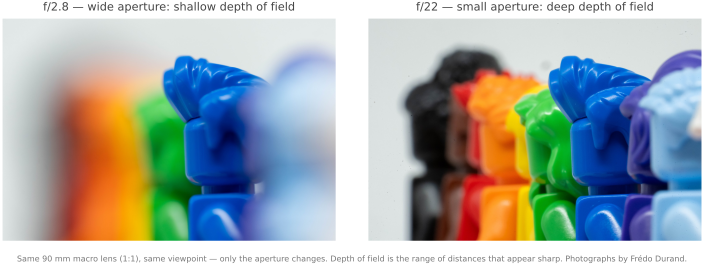
2.9.1 The circle of confusion⧉
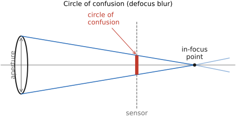
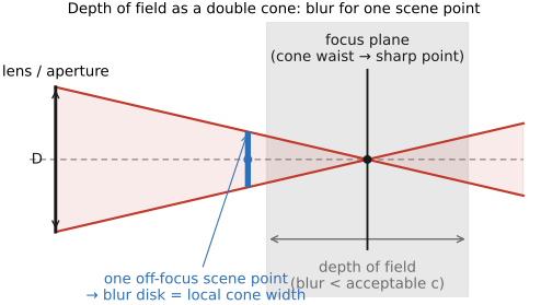
Start with one out-of-focus point (Figure 2.9.2). A point at the focus distance sends a cone of rays through the lens that reconverges exactly on the sensor, a sharp point. A point too far away focuses in front of the sensor, so by the time its cone reaches the sensor it has opened back up into a small disk; a point too near focuses behind the sensor and likewise lands as a disk. That blur disk is the circle of confusion. A point still counts as "sharp" as long as its circle of confusion stays smaller than some acceptable diameter $c$, set by the sensor's resolution and how large you will view the print (for 35 mm film, $c$ is traditionally about 0.02 mm). The disk grows with the aperture (a wider opening, a fatter cone, a bigger disk) and with the point's distance from the focus plane (zero exactly at focus, growing both ways) (Figure 2.9.3).
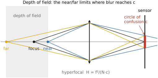
A defocused point never images as a point but as a blur disk: the circle of confusion. The depth of field is then defined as the range of distances over which that disk stays smaller than a chosen maximum $c$: inside the depth of field every point is blurred less than $c$, outside it more. The operative word is acceptable: $c$ is not a constant of nature but a judgement call that depends on the target application, the viewing distance, and the sensor (or print) resolution. A billboard read from across the street tolerates a huge $c$; a 100% crop on a 4K monitor almost none. Change the standard and the depth of field changes with it, even though the optics did not.
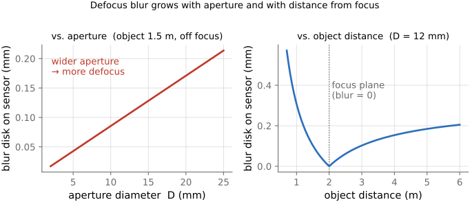
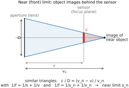
The formula. All of this is one short calculation. Focus at distance $s$, so the lens (aperture diameter $D = f/N$) images the focus plane sharply onto the sensor. A point at some other distance $d$ would focus at a slightly different image distance, so its cone reaches the sensor still open, as a disk. Following that cone by similar triangles (the image-side construction of Figure 2.9.8) and eliminating the image distances with the thin-lens conjugate relation $1/f = 1/v + 1/d$ gives the circle of confusion as a function of the point's distance:
Everything qualitative reads straight off it: the blur is exactly zero at $d = s$ (the focus plane), grows with the focal length squared, grows as the aperture opens (small $N$), and grows with how far the point strays from focus. For a subject far compared with the focal length, $s - f \approx s$ and it simplifies to the approximate form
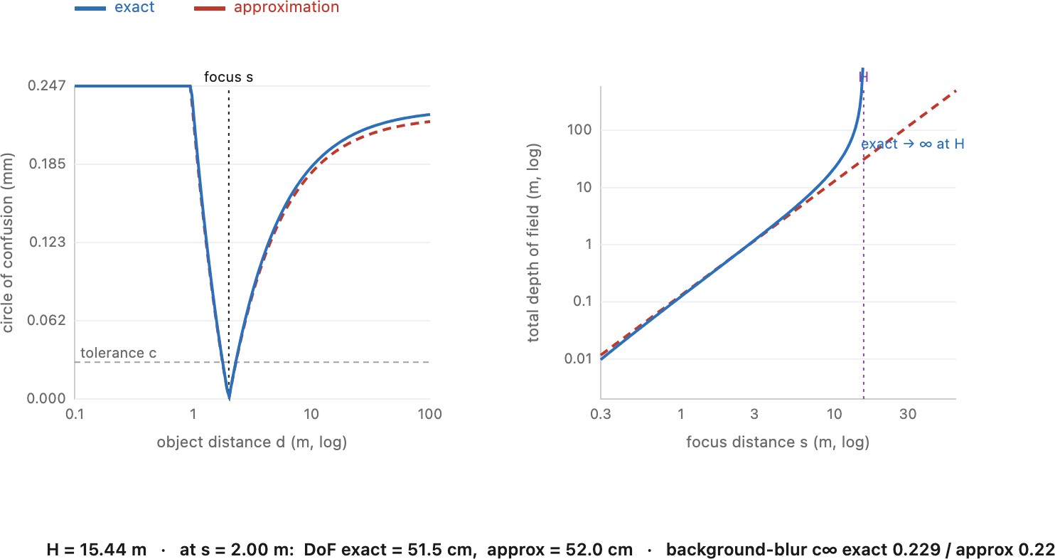
The two agree to well under a pixel for ordinary photography and part company only in the macro range, where $s$ approaches $f$ (Big lesson L2.35). One special case is worth keeping: a background at infinity ($d \to \infty$, so $\lvert s-d\rvert / d \to 1$) blurs to $c_\infty \approx f^2/(N s)$, which equals the tolerance $c$ exactly when $s$ is the hyperfocal distance $H = f^2/(N c)$. That coincidence, background-blur-equals-tolerance at $s = H$, is the tie we exploit below.
2.9.2 Depth of field versus depth of focus⧉
The circle of confusion has two faces, and it is worth separating them because they are easy to confuse (the names differ by one word). Depth of field is the object-side story we have been telling: with the sensor fixed, it is the range of subject distances that image acceptably sharply. Depth of focus is its image-side mirror: with the subject fixed, it is the range of sensor positions that keep that subject acceptably sharp, the mechanical tolerance on where the sensor (or film) is allowed to sit behind the lens. One lives out in the world in front of the lens; the other lives in millimeters, or rather microns, behind it.
They are conjugates, tied by the magnification. On the image side the tolerance is simply $2Nc$ (the blur cone reaches the tolerance $c$ when the sensor is displaced by $\pm N c$ either way), essentially independent of subject distance; project that image-side band back out through the lens and you get the object-side depth of field, which is why the latter stretches so dramatically with distance while the former barely moves. The practical weight is all on how small depth of focus is: at $f/2$ with $c \approx 0.02$ mm it is only about $\pm 0.04$ mm, so the sensor must be positioned, held flat, and kept parallel to that tolerance, and an autofocus system must place the focus to it. This is exactly why fast lenses demand tighter mechanical precision, why sensor flatness and film flatness matter, and why back- or front-focus of even a fraction of a millimeter is visible wide open but forgiven when stopped down (larger $N$ widens the depth of focus in proportion). Same geometry, two sides of the lens: depth of field is the photographer's concern, depth of focus the camera engineer's.
2.9.3 Choosing the maximum circle of confusion⧉
The whole depth-of-field machinery hangs on one number, the tolerance $c$, and the big lesson above already warned that it is a judgement, not a constant. It is worth being concrete about how that judgement has actually been made, because there are three different conventions and they answer three different questions.
The classic version. Before digital, $c$ was pinned to a standard viewing scenario: enlarge the negative to a normal print (about 8×10 inches), view it at a comfortable distance (roughly the print's own diagonal, ~25–30 cm), and assume the eye resolves about 5 line-pairs per millimetre there. Trace that back through the enlargement and you get a fixed circle of confusion on the film or sensor, and the rule of thumb that survives is $c \approx \text{(sensor diagonal)}/1500$, about 0.02–0.03 mm for full-frame. Every depth-of-field scale ever engraved on a lens, and every online DoF table, quietly bakes in this one scenario. Its virtue is a single number per format; its vice is that it is wrong the moment you view the image any other way.
Pixel size. A digital-native alternative ignores viewing entirely and sets $c$ to a small multiple of the pixel pitch, often just one or two pixels. This is the right tolerance when the file itself is the product, judged at 100% on a monitor, or fed to a matching or reconstruction algorithm: a blur smaller than a pixel cannot be recorded anyway, so anything under a pixel is automatically "sharp." It ties depth of field to the sensor's resolution rather than to any print.
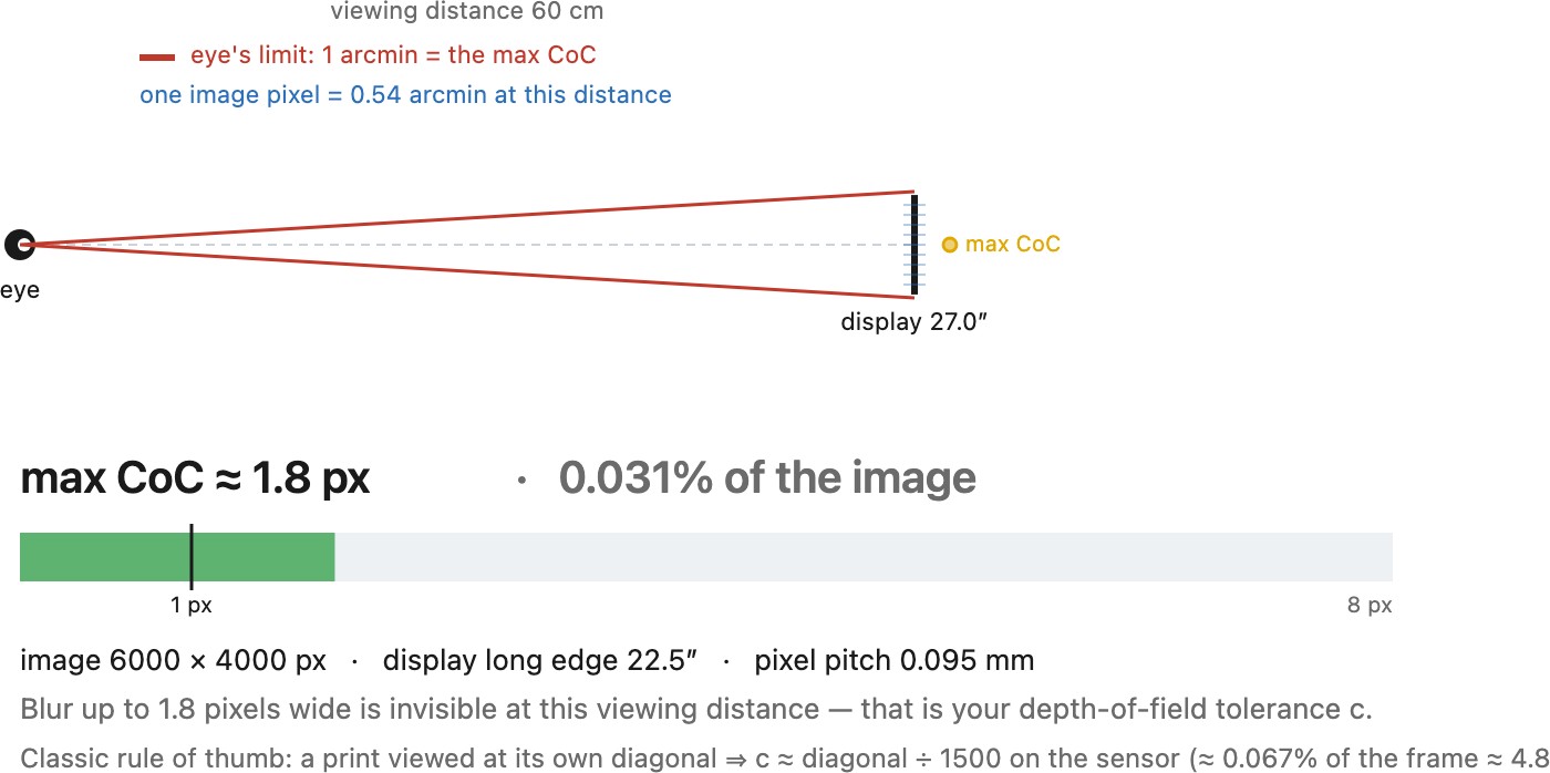
Different display conditions. Both of the above are special cases of the only definition that is really true: $c$ is set by whatever blur is just too small to see in the final image, as it is actually viewed. A billboard read from across the street, a phone at arm's length, and a 100% crop on a 4K monitor differ by orders of magnitude in the tolerance they allow, from the same negative. The clean way to compute it is to work in the viewing geometry directly. The eye resolves about one arcminute; a blur on the display that subtends less than that is invisible. So from the display size, the viewing distance, and the image's pixel count you can read off the largest circle of confusion that still looks sharp, in image pixels or as a fraction of the frame, with the classic $\text{diagonal}/1500$ falling out as the one frozen standard (Figure 2.9.4). Set $c$ from your output, not from a table built for someone else's print.
2.9.4 The double cone, and the near and far limits⧉
The simplest picture lives in object space: a double cone in front of the lens, its waist sitting on the focus plane, whose width at any depth is the blur that a point there would produce (Figure 2.9.6). Depth of field is the range of object distances whose circle of confusion stays within $c$, bounded by a near limit (closest still-sharp distance) and a far limit (farthest). The derivation is the same similar-triangles move as above, now solved the other way: take the circle-of-confusion formula, set $c(d) = c$, and solve for the object distance $d$. Because $c(d)$ carries $d$ in its denominator, that is a quadratic, and its two roots are the near and far limits (Figures 9, 10, and 11). Written with the hyperfocal distance $H = f^2/(N c) + f$ they take their standard compact form
with $D_f = \infty$ as soon as $s \ge H$: the far limit has run off to infinity, which is exactly what singles $H$ out. The total depth of field is $D_f - D_n$. Dropping the small $-f$ and $-2f$ terms (the same $s \gg f$ assumption) tidies these to
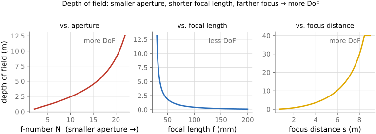
and one further step, for a subject much closer than the hyperfocal distance ($s \ll H$), collapses the total to the memorable scaling of the next lesson, $\text{DoF} \approx 2 N c\,s^2/f^2$. That last form is the one to carry around, and also the most approximate: it assumes both $s \gg f$ and $s \ll H$, so it is faithful across the everyday portrait-to-landscape middle and wrong at both ends, collapsing too fast in macro and, more visibly, missing the runaway to infinity as $s$ approaches $H$. The exact limits and their approximations are plotted together in Figure 2.9.10: the curves lie on top of each other across the ordinary range and split apart precisely where the assumptions fail. One caveat the tidy formulas hide is that the depth of field is asymmetric, with more sharp depth behind the focus plane than in front (the "roughly one third in front, two thirds behind" rule of thumb), and that asymmetry only grows with distance until the far limit reaches infinity. The qualitative results, though, are what you carry around, and they all point the same way: depth of field grows with a smaller aperture (larger $N$), a shorter focal length, and a greater focus distance (Figure 2.9.9). Stopping down is the photographer's main knob, but it costs light, so it forces a longer exposure or a higher ISO (more noise), and stopped down too far, diffraction softens everything (previous part). You can only push it so far.
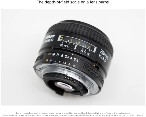
Before calculators, all of this was engraved on the lens itself (Figure 2.9.5). The depth-of-field scale on a manual-focus barrel is a mechanical solution of exactly these near- and far-limit equations: two mirrored rows of f-numbers straddle the focus index, and for a chosen aperture its two marks bracket the near and far distances that will be sharp. Wider apertures give a narrow pair of marks (shallow depth), smaller apertures a wide pair, and setting the far mark on the infinity symbol is how you dial in the hyperfocal distance of the next section by hand.
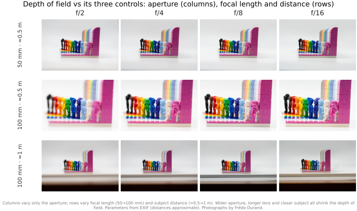
Away from the macro range (subject much closer than the hyperfocal distance), the total depth of field follows a clean scaling, $\text{DoF}\approx \dfrac{2\,N\,c\,s^2}{f^2}$: it grows linearly with the f-number $N$ (stop down for more), quadratically with the focusing distance $s$ (step back and it balloons), and inversely with the square of the focal length $f$ (wider for more, longer for less). These three exponents explain at a glance why a phone (tiny $f$) keeps almost everything sharp, why close focus annihilates depth of field, and why "I need more in focus" always reduces to stop down, back up, or go wider.
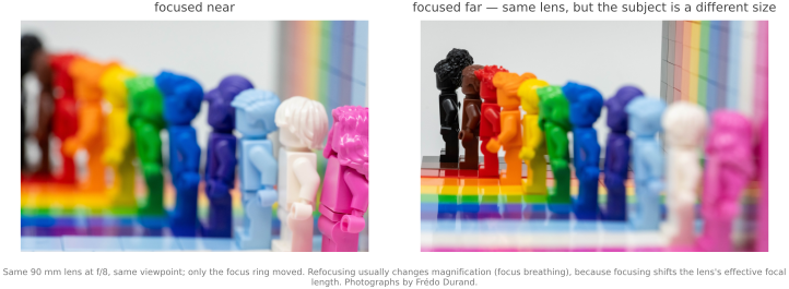
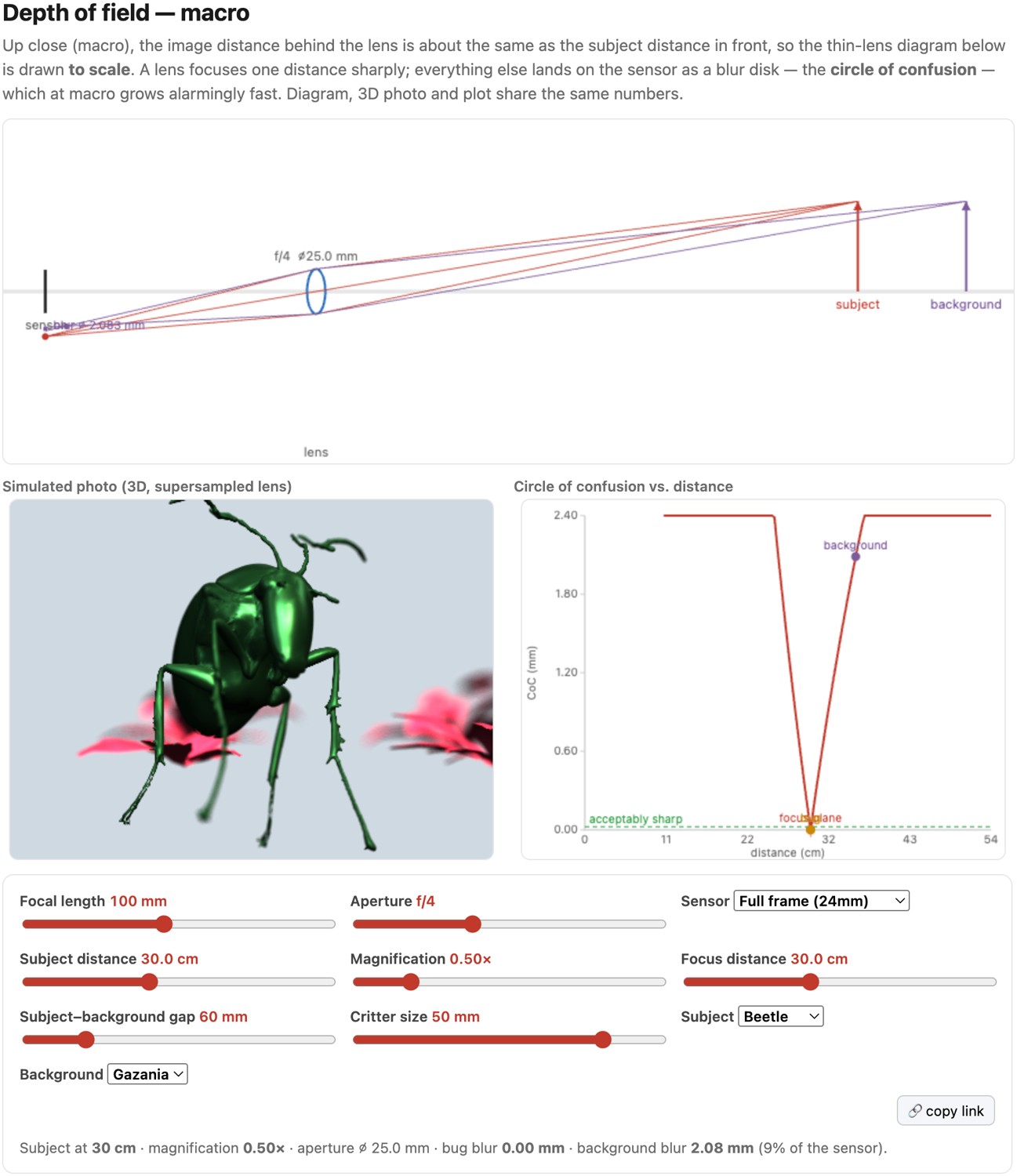
The convenient first-order results of this chapter (the depth-of-field scaling just above, the framing shortcut "magnification $\approx f/\text{distance}$", even the bare f-number as a stand-in for image brightness) all quietly assume the subject is far compared with the focal length. Up close (macro, at magnifications near or past 1:1) they break. The pupil magnification stops being 1, the effective f-number grows as $N(1+m)$ so you lose real light, the working distance shrinks toward the front element, and the depth of field collapses to millimeters. In the macro regime you must drop the shortcuts and return to the exact conjugate geometry (and, often, to focus stacking). It is a good reflex to ask of any optics approximation: does this still hold when the subject is this close?
2.9.5 Hyperfocal distance⧉
There is one focus setting that wrings the maximum depth of field out of a lens. Focus at the hyperfocal distance
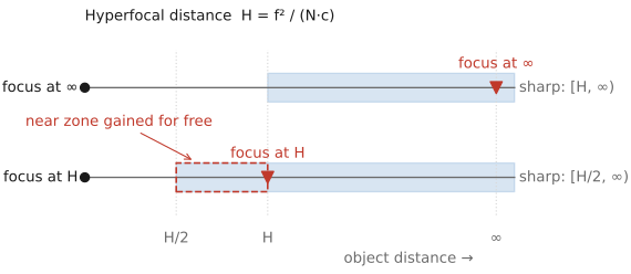
and everything from $H/2$ all the way to infinity falls within the tolerance $c$ (Figure 2.9.12). This is the landscape photographer's trick (Ansel Adams used it constantly): focusing at infinity instead wastes the whole sharp zone between $H/2$ and $H$, whereas focusing at $H$ buys it back for free.
This is also the principle behind fixed-focus cameras, which have no focusing mechanism at all: the lens is simply glued at (or just beyond) the hyperfocal distance so that everything from $H/2$ to infinity is acceptably sharp. Because $H = f^2/(Nc)$ shrinks with the square of the focal length, this is easy when $f$ is tiny, which is exactly why it works so well for the short focal lengths of disposable cameras, webcams, doorbell and security cameras, and the ultra-wide modules on phones, and why those wide phone cameras can skip autofocus entirely while their longer (tele) modules cannot. The cost is that you can never throw the background out of focus or focus closer than $H/2$; fixed focus trades away near-subject sharpness and selective focus for a camera with no moving parts.
There is a single focus setting that extracts the maximum depth of field from a lens: the hyperfocal distance $H = f^2/(N c)$. Focus there and the far limit runs all the way to infinity while the near limit sits at exactly $H/2$, so the entire scene from $H/2$ to the horizon falls inside the acceptable circle of confusion. Focusing at infinity instead throws away the whole sharp zone between $H/2$ and $H$ for nothing. It is the landscape-and-street photographer's standard move for front-to-back sharpness, and the basis of zone focusing (pre-set the focus, shoot without refocusing).
2.9.6 The surprising invariance⧉
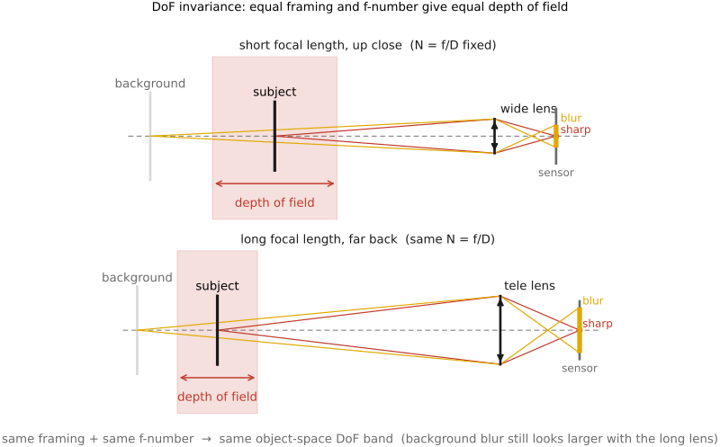
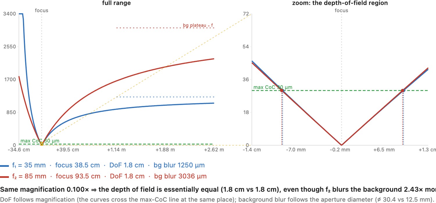
The practical conclusion is that a longer focal length does not, by itself, reduce depth of field when framing and f-number are held fixed. "Telephoto lenses have shallow depth of field" is not really true as stated. For a fixed framing (you keep the subject the same size in the frame) and a fixed f-number, the depth of field in object space is essentially independent of focal length (Figure 2.9.13). Switch from a 28 mm to a 100 mm lens and, to keep the subject the same size, you must step back; stepping back deepens the depth of field by exactly as much as the longer focal length shrinks it, and the larger physical aperture of the long lens (same f-number $N = f/D$ means $D$ grew with $f$) cancels the rest. The two effects exactly compensate. So shallow depth of field is really about magnification (how large the subject is on the sensor), not focal length per se.
This is genuinely useful: for macro work, where depth of field is precious, you can change your working distance (back off to make room for lights, say) without changing the depth of field at all, as long as you re-frame to the same magnification. The background does still look more blurred through the long lens, but that is because the long lens magnifies the already-out-of-focus background disks, not because the depth-of-field band changed.
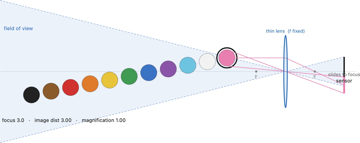
All of this (the three controls, the circle of confusion, the near/far limits, the hyperfocal distance, and the constant-magnification invariance) is easiest to feel by driving it yourself (Figure 2.9.16). It is the same physics as the 3-D macro simulator at the end of this chapter, drawn as a single 2-D ray diagram plus a plot, so the numbers are right there: slide the focal length, f-number, and subject distance and watch the near/far limits and $H$ move; then tick constant magnification and watch the depth of field go nearly flat against focal length, the invariance of the previous paragraph, made literal.
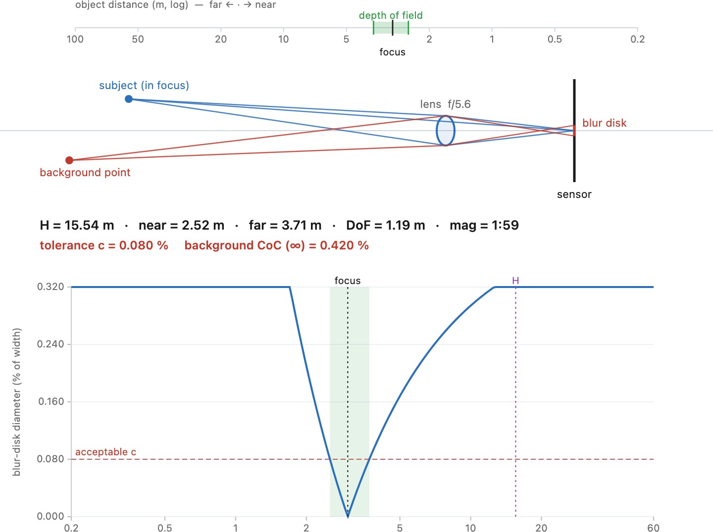
The invariance is sharpest when you plot two focal lengths at once (Figure 2.9.17). Fix the magnification (the same framing of the subject) and draw the circle of confusion against distance from the focus plane for a short and a long lens: around the focus the two curves coincide, so the depth of field is the same, but far behind the subject the long lens climbs to a much higher plateau. That plateau is the background blur, and it equals the aperture diameter times the magnification ($f\,m/N$), so it grows with focal length. Depth of field is set by magnification; how hard a distant background is thrown out of focus is set by the aperture diameter. The two facts live in the same picture.
2.9.7 Background blur beyond the focus plane⧉
The invariance is a statement about the near neighborhood of the focus plane: hold the framing and two focal lengths give the same depth of field. Push past that neighborhood, out toward the background, and the two lenses part company. The circle of confusion keeps growing with distance from the focus plane, and it grows faster for the longer lens, until it saturates at a ceiling set by a subject infinitely far away. That ceiling is the background blur, the quantity that decides how cleanly a portrait separates from its backdrop, and it is worth deriving on its own.
The infinity blur. Take the circle of confusion of the previous sections and let the object recede to infinity. With the subject focused at $s$,
because $\lvert d-s\rvert / d \to 1$. This is the on-sensor blur diameter of a point infinitely far behind the subject. It has a clean reading once you substitute the aperture diameter $D=f/N$ and the on-axis magnification $m=f/(s-f)$:
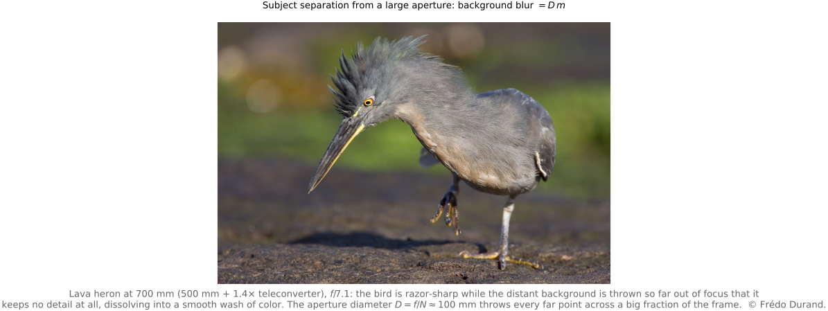
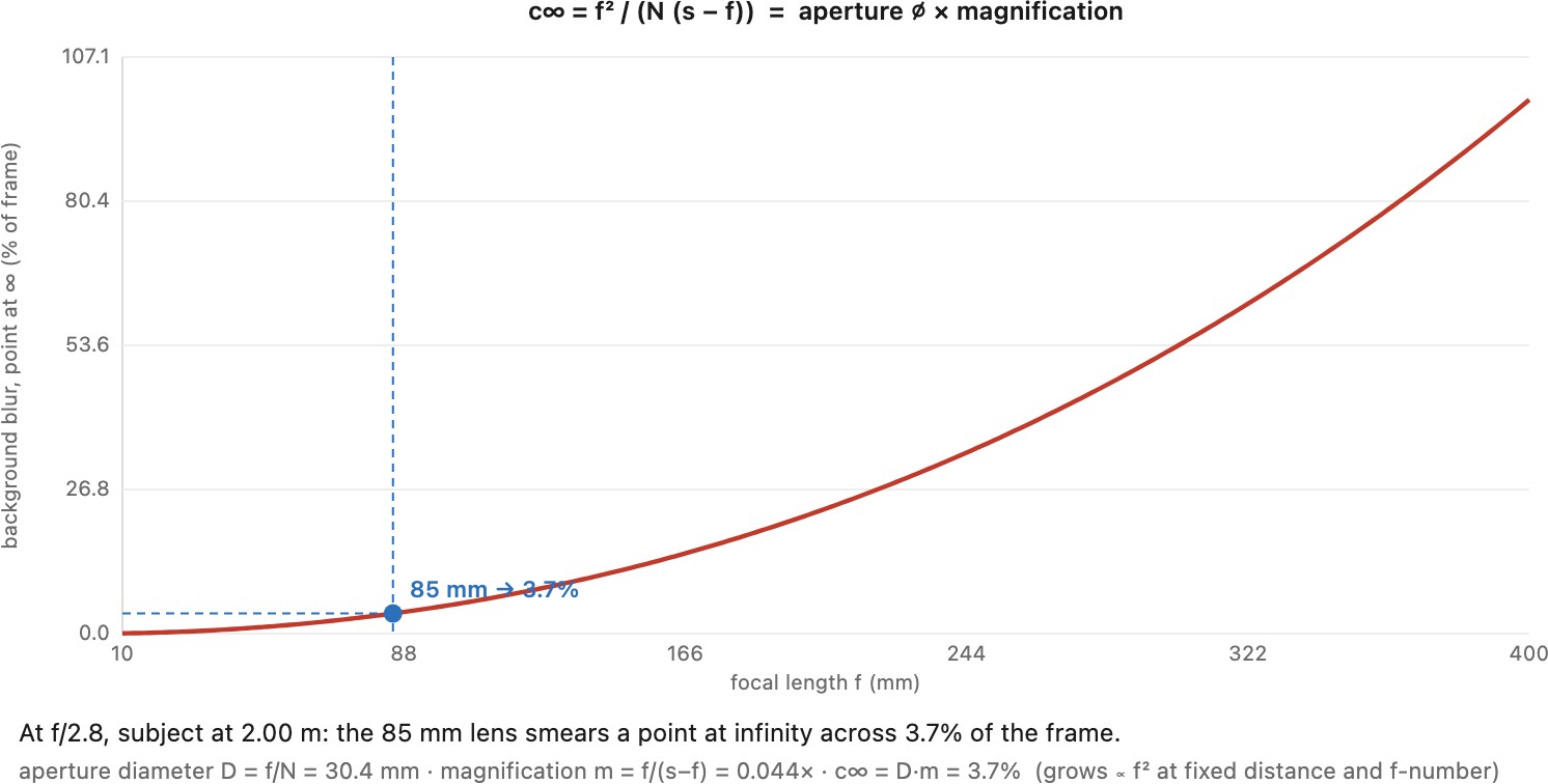
the aperture diameter times the magnification, the same $f\,m/N$ plateau the two-focal-length figure climbed to. Read it two ways. At a fixed framing (fixed $m$) it scales with the physical aperture $D$, which is the sensor-size argument of the next section: a bigger lens throws a background further out of focus. At a fixed subject distance $s$, which is what a photographer swapping lenses on the spot actually holds, it scales as $f^2/(s-f)$, close to $f^2$ for an ordinary subject, so doubling the focal length roughly quadruples the background blur. That is the real content of "telephotos blur the background": it is a claim about the background, not about the depth of field, which the previous section showed is unchanged at fixed framing. A big super-telephoto, with its large physical aperture, is where this reaches its extreme (Figure 2.9.18): a distant background collapses into a smooth wash, isolating the subject completely.
To compare $c_\infty$ against a tolerance, divide by the sensor width $w$ for a fraction of the frame, or multiply by the horizontal pixel count $n_\text{px}$ for pixels:
The background blur is thus fixed by five numbers: the f-number, the focal length, the focus distance, the sensor size, and (for pixels) the resolution. Figure 2.9.19 plots it against focal length at a chosen f-number and distance, and the near-$f^2$ climb is the whole story.
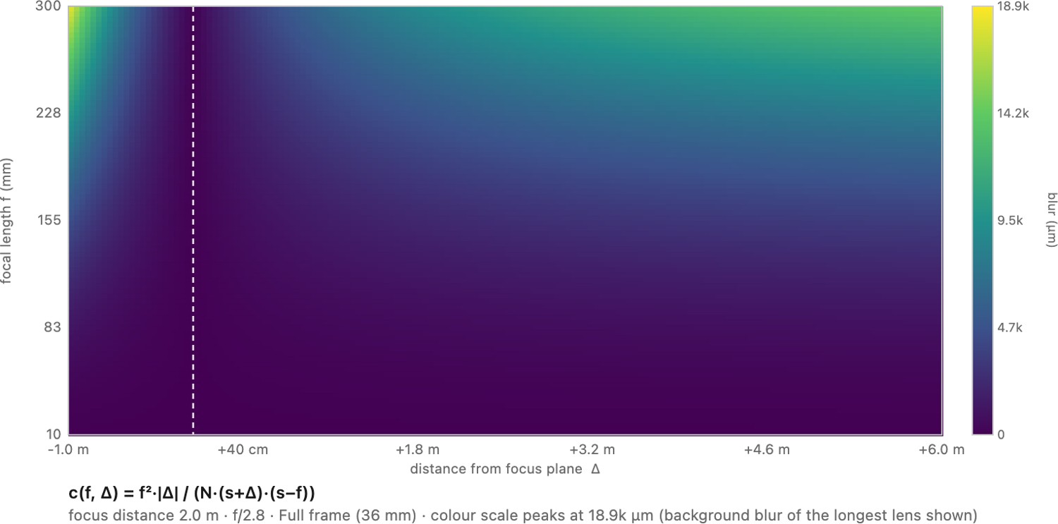
The whole field. The infinity blur is one edge of a two-dimensional picture. Hold the f-number and the focus distance and the full circle of confusion is a function of two variables at once, the focal length and the signed distance from the focus plane $\Delta = d - s$ (background positive, foreground negative):
Figure 2.9.21 draws this field, as a colour map or a spinnable 3-D surface. Two features carry the depth-of-field story in one image. Along $\Delta=0$ runs a valley of zero blur, the focus plane. Its slope, the rate at which blur opens up as you leave focus, is $\lvert\partial c/\partial\Delta\rvert$ at $\Delta=0$, which reduces to
depending only on the magnification and the f-number, not on the focal length. That is the invariance, made into a tangent: at a given framing every focal length shares the same ridge slope at the valley, so the same near-focus depth of field. Away from focus the surface climbs, and it climbs steeper for larger $f$, so the curves for two focal lengths, tangent at the valley, separate as $\Delta$ grows and level off at the infinity ceiling $c_\infty = f^2/(N(s-f))$ derived above. Depth of field lives in the tangent; background blur lives in the plateau; the one surface holds both.
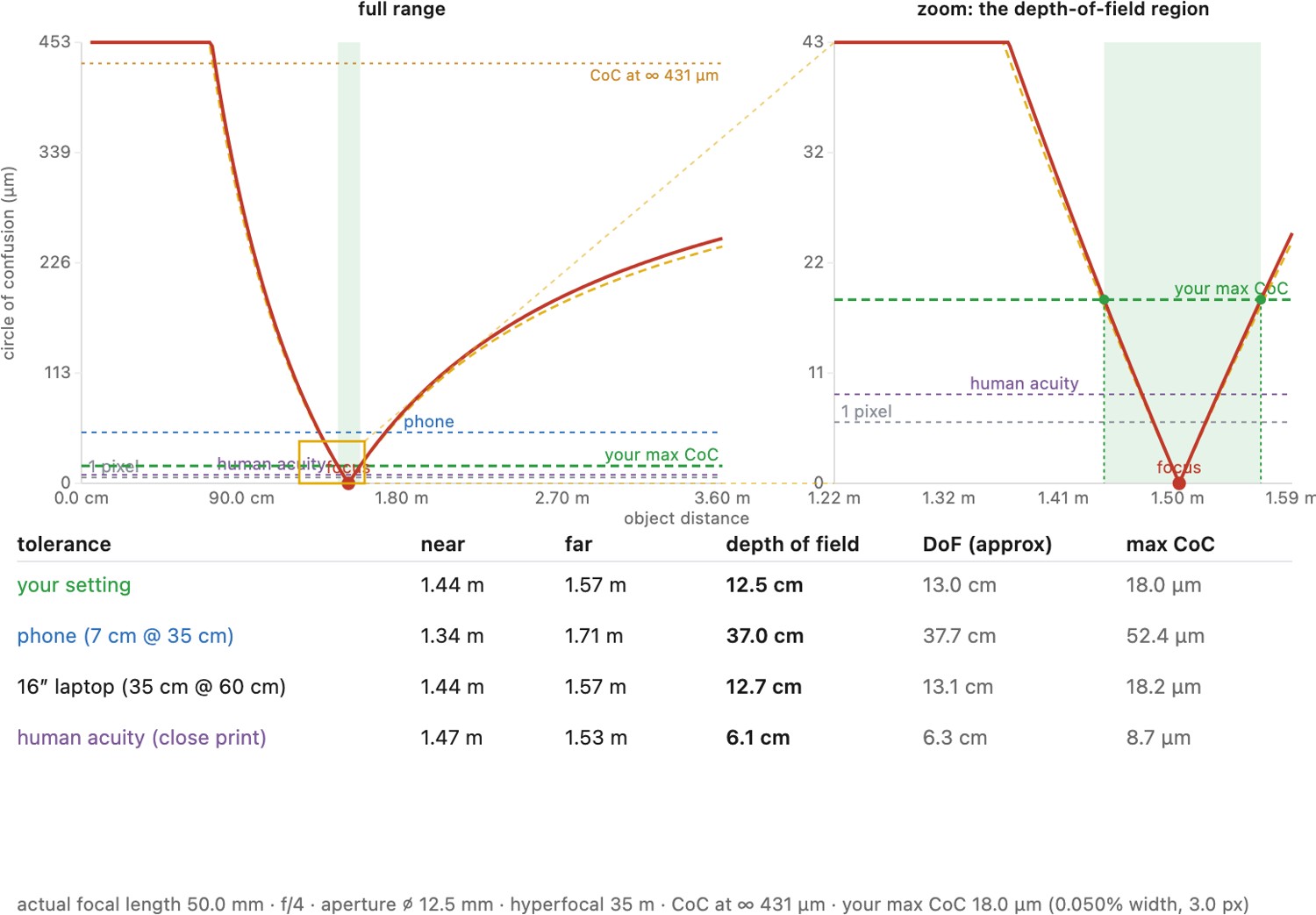
The calculator. All of this (the exact circle of confusion and its far-subject approximation, the near and far limits, the hyperfocal distance, the infinity blur, and the tolerance that turns a blur into a depth of field) gathers into one working tool in Figure 2.9.22. Set the focal length (as a 35 mm-equivalent, so the framing is held fixed as you change sensors), the f-number, the focus distance, the sensor, and your acceptable circle of confusion in pixels or percent of the frame. It draws the circle of confusion against distance, marks the infinity blur and the tolerances a single pixel, a phone, and the eye's acuity each imply, and reads the depth of field off at your setting and at typical phone and 16-inch-laptop viewing, giving both the exact thin-lens value and the $2Ncs^2/f^2$ approximation side by side. The tangent near focus is where the depth-of-field invariance lives; the growth beyond it, out to the infinity plateau, is the background blur. It is the calculator form of the one idea this chapter keeps returning to: the depth of field is only as real as the maximum circle of confusion you are willing to accept, and that number comes from how the picture will be seen.
2.9.8 Defocus is not a blur of the image⧉
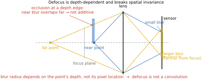
It is tempting to think you could fake shallow depth of field by simply blurring a sharp photo, convolving it with a disk. You cannot, and the reason matters (Figure 2.9.23). The circle of confusion depends on each point's scene depth, not on its position in the image, so the blur is spatially varying in a way tied to 3D structure rather than pixel coordinates. Worse, at depth discontinuities (the edge of a foreground object against a far background) occlusion comes into play: the blurred foreground should bleed over the background, and the background that the foreground hides should partly show through the foreground's blur, neither of which a flat 2D blur can do. Depth of field is not a convolution of the image. This is exactly why naive "portrait mode" fakes look wrong at hair and edges, and why depth-aware and light-field methods (Advanced part), which know each pixel's depth, or capture the rays directly, do so much better.
2.9.9 Sensor size scales depth of field⧉
Finally, a fact that explains your phone. Shrink the sensor while keeping the field of view (FOV), and both the circle of confusion $c$ and the physical aperture $D$ shrink in proportion, so depth of field grows linearly as the sensor shrinks. Phone cameras therefore have enormous depth of field: almost everything is in focus, which is why they must fake background blur computationally (portrait mode). The same fact makes macro photography easier on small sensors: a scaled-down camera photographs a scaled-down world, gaining both closer minimum focus and more depth of field for free, except for diffraction, since shrinking the camera does not shrink the wavelength of light.
The same story told from the image side is the one a phone designer feels most acutely. For a subject held at a fixed framing, the out-of-focus blur of the background (measured as a fraction of the frame) is proportional to the lens's physical aperture diameter $D = f/N$. Scale the whole camera down by the crop factor (sensor and focal length shrink together, the f-number $N$ held fixed) and $D$ shrinks by that same factor, so the background blur shrinks linearly with the sensor. A phone, whose sensor is roughly seven times smaller than full frame, therefore produces about seven times less background blur at the same f-number, which is exactly why it cannot throw a background out of focus and must synthesize shallow depth of field in software (portrait mode; the computational treatment is a later chapter). Put as equivalence: a phone at $f/1.8$ has the depth of field of a full-frame lens at roughly $f/12$.
Hold the framing and the f-number fixed and scale the camera down: the defocus blur of the background, as a fraction of the frame, shrinks linearly with the sensor size, because it tracks the lens's physical aperture diameter $D=f/N$ and $f$ shrinks with the sensor. So shallow depth of field is a privilege of physically large apertures (a big sensor with a big lens) and a small sensor cannot fake it optically. This is why phones have deep depth of field and must compute fake background blur (portrait mode, a later chapter): the tiny sensor shrinks every blur disk toward nothing. It is the image-space twin of "small sensor → more depth of field" above.
A revealing optical workaround predates the computational one: relay optics. Place a physically large lens out front to cast a large, genuinely shallow-depth-of-field image onto a diffusing ground-glass screen, then re-photograph that screen with a small-sensor camera through a macro/relay lens. The small camera now inherits the big lens's shallow depth of field (and its wide field of view), paying only in lost light, a little softness, and the screen's faint grain. This is precisely how 35 mm lens adapters (the Letus, Redrock M2, and Brevis units, and the older Frazier-style relays) let early small-sensor camcorders (and the first video-DSLR rigs) borrow a large-format "cinematic" look before big-sensor video existed; the same relay trick lives on in view-camera ground glass and in microscope-to-camera couplings.
Recap: big lessons of this chapter
A defocused point never images as a point but as a blur disk: the circle of confusion. The depth of field is then defined as the range of distances over which that disk stays smaller than a chosen maximum $c$: inside the depth of field every point is blurred less than $c$, outside it more. The operative word is acceptable: $c$ is not a constant of nature but a judgement call that depends on the target application, the viewing distance, and the sensor (or print) resolution. A billboard read from across the street tolerates a huge $c$; a 100% crop on a 4K monitor almost none. Change the standard and the depth of field changes with it, even though the optics did not.
Away from the macro range (subject much closer than the hyperfocal distance), the total depth of field follows a clean scaling, $\text{DoF}\approx \dfrac{2\,N\,c\,s^2}{f^2}$: it grows linearly with the f-number $N$ (stop down for more), quadratically with the focusing distance $s$ (step back and it balloons), and inversely with the square of the focal length $f$ (wider for more, longer for less). These three exponents explain at a glance why a phone (tiny $f$) keeps almost everything sharp, why close focus annihilates depth of field, and why "I need more in focus" always reduces to stop down, back up, or go wider.
The convenient first-order results of this chapter (the depth-of-field scaling just above, the framing shortcut "magnification $\approx f/\text{distance}$", even the bare f-number as a stand-in for image brightness) all quietly assume the subject is far compared with the focal length. Up close (macro, at magnifications near or past 1:1) they break. The pupil magnification stops being 1, the effective f-number grows as $N(1+m)$ so you lose real light, the working distance shrinks toward the front element, and the depth of field collapses to millimeters. In the macro regime you must drop the shortcuts and return to the exact conjugate geometry (and, often, to focus stacking). It is a good reflex to ask of any optics approximation: does this still hold when the subject is this close?
There is a single focus setting that extracts the maximum depth of field from a lens: the hyperfocal distance $H = f^2/(N c)$. Focus there and the far limit runs all the way to infinity while the near limit sits at exactly $H/2$, so the entire scene from $H/2$ to the horizon falls inside the acceptable circle of confusion. Focusing at infinity instead throws away the whole sharp zone between $H/2$ and $H$ for nothing. It is the landscape-and-street photographer's standard move for front-to-back sharpness, and the basis of zone focusing (pre-set the focus, shoot without refocusing).
Hold the framing and the f-number fixed and scale the camera down: the defocus blur of the background, as a fraction of the frame, shrinks linearly with the sensor size, because it tracks the lens's physical aperture diameter $D=f/N$ and $f$ shrinks with the sensor. So shallow depth of field is a privilege of physically large apertures (a big sensor with a big lens) and a small sensor cannot fake it optically. This is why phones have deep depth of field and must compute fake background blur (portrait mode, a later chapter): the tiny sensor shrinks every blur disk toward nothing. It is the image-space twin of "small sensor → more depth of field" above.