2.8 Image measurements as integrals🔗⧉

A camera makes a number out of light. Point it at a scene, open the shutter, and where there was a continuous, infinitely detailed field of light there is now a grid of integers. The question of this chapter is exactly what each of those integers is — what physical quantity a pixel value reports, and what governs how trustworthy it is.

A pixel value is an integral of the incoming light over aperture, sensor area, wavelength, and time. The light reaching the camera is not one ray but a whole bundle, spread over a range of directions (the aperture), a patch of the sensor (the pixel's area), a band of colors (wavelength), and a stretch of time (the exposure). The sensor adds all of it up. The rest of the chapter elaborates that statement: first by naming the full field of light a camera draws from (the plenoptic function), then by writing the measurement itself as that integral and connecting its four axes to the camera's controls, and finally by describing the physical device that performs it (the sensor). The inevitable jitter in the result — noise — traces straight back to the fact that the thing being integrated is a stream of discrete, randomly arriving photons; it is the subject of the next chapter.

2.8.1 The plenoptic function🔗⧉

Before we can say what a pixel measures, it helps to name everything there is to measure. Stand in a room and ask: what is all the light here, before any camera, eye, or sensor selects from it? At every point in space, light is passing through in every direction, at every wavelength, at every instant. The function that captures all of it at once is the plenoptic function (from plenus, full, and optic, literally "full optic") introduced by Adelson and Bergen.

Parameterize a single ray of light by its 3D position $(x, y, z)$, its 2D direction $(\theta, \phi)$, its wavelength $\lambda$, and the time $t$, and the plenoptic function returns the radiance carried by that ray:

That is seven numbers in and one radiance out: a seven-dimensional description of every ray of light filling all of space, in every direction and color, at every moment. It is everything there is to see, from everywhere, at once (Figure 2.8.1).

There is a deeper lesson in Adelson and Bergen's paper that is usually forgotten — it tends to be cited only for naming the function. Their real argument was that early vision is, throughout, the measurement of the local structure of $P$, and that the same operations, such as local averages, derivatives, and oriented filters, recur along every axis: a spatial edge, a temporal event, a binocular disparity, and a motion are all the visual system taking derivatives of the plenoptic function along different dimensions. Low-level vision is essentially one kind of task, repeated across space, time, viewpoint, and wavelength. That unifying view echoes through this book on the camera side too, because many photographic scenarios are the same operation along a different axis of $P$. A light-field (plenoptic) camera samples variation across the aperture exactly as a high-speed video camera samples variation across time — both densely slice the plenoptic function along one of its axes and resolve afterwards what a conventional camera integrated away (→ 14 Light fields and plenoptic cameras, 11 Multiple exposure imaging, and the capture-the-set-decide-later lesson L11.2). Keeping the whole function in view is what makes those parallels visible.

Seven is the classical count, and it captures everything an ordinary camera responds to — but a ray of light carries one more property the standard plenoptic function omits: its polarization, the orientation in which the light's electromagnetic field oscillates. Add it as an eighth axis and $P$ gains a polarization argument. We are largely blind to it, so it is easy to forget; yet it is physically there on every ray, and it is information — the sky is partially polarized in a pattern that follows the sun, reflections off glass and water are strongly polarized (which is how a polarizing filter cuts glare), and the surface orientation of an object leaves a polarization signature. Many animals read it directly (bees navigate by the sky's polarization pattern; mantis shrimp even sense circular polarization — see Animal eyes), and polarization cameras sample it on purpose for glare removal, reflection separation, and shape-from-polarization. It is one more dimension of the light that a measurement can choose to integrate over (throwing it away, as most sensors do) or resolve (as a polarization camera does) — the same capture-or-discard choice the rest of this chapter draws for direction, wavelength, and time.

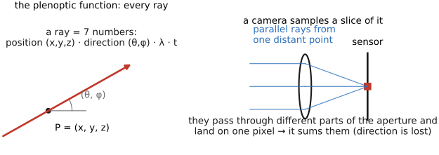
The reason to introduce such an extravagant object is that it makes one idea precise: any imaging operation is the measurement of some portion of the plenoptic function. The eye samples a 2D slice; a video camera samples a 2D slice that also varies over time; a depth sensor recovers part of the geometry hidden in it; a light-field camera grabs a richer 4D chunk. Each imaging device is just a different way of sampling $P$.

In particular, a conventional camera records only a 2D projection. Each pixel collects all the rays that reach it through the aperture and sums them, discarding their direction — it keeps the total arriving light, not the direction within the aperture from which it came. That discarded directional information — the radiance as a function of which direction within the aperture each ray came from — is exactly the 4-D light field, and recording it instead of summing it away is what light-field and multi-aperture cameras do, so they can refocus, change aperture, or shift viewpoint after the shot (14 Light fields and plenoptic cameras). For an ordinary camera it is thrown away, and the throwing-away is an integral. The next section makes that literal.

2.8.2 The pixel integral🔗⧉

The plenoptic function now pays off concretely. We said a conventional camera measures only a 2D projection of $P$; we can now say exactly what each pixel of that projection holds. A pixel does not sample a single ray; it integrates a slice of $P$ over four plenoptic dimensions at once, each weighted by how the pixel responds there (Figure 2.8.2):

1. the aperture — all the ray directions $(\theta, \phi)$ the lens admits toward this pixel, a solid angle set by the f-number;
2. the pixel's area $(x, y)$ on the sensor — a finite patch, not a mathematical point;
3. wavelength $\lambda$ — weighted by the sensor's and color filter's spectral response; and
4. the exposure time $t$ — the interval the shutter is open.

Schematically, the value recorded at a pixel is

the scene radiance integrated over aperture × pixel area × wavelength × time, weighted by the pixel's spectral response $r(\lambda)$ and the geometric weight $k$ that the aperture and footprint impose. Stated in one line: measurement is integrating the plenoptic function against the pixel's sampling kernel — and the support of that kernel along each axis is exactly a photographic knob. Because the underlying capture counts photons, this integral is linear in scene radiance — a fact we will need both for high-dynamic-range merging and for the noise analysis later in the chapter.

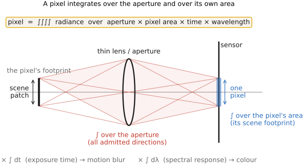
The four domains are the four knobs. What makes this more than bookkeeping is that each integration domain is governed by a control the photographer actually sets — the integral is the camera's exposure settings, written as mathematics:

• the aperture integral is set by the f-number $N = f/D$: stopping down shrinks the cone of directions each pixel sums over (less light, more depth of field); opening up widens it;
• the exposure-time integral is set by the shutter speed: a longer interval integrates over more time (more light, but more motion blur);
• the pixel-area integral is fixed by the sensor's pixel pitch — the physical size of a photosite — which is why a larger sensor (or larger pixels) gathers more light per pixel, trading against spatial resolution;
• the wavelength integral is shaped by the spectral response — the sensor's sensitivity curve times the color filter over each photosite — which collapses a whole spectrum into a single number per channel.

The one familiar exposure control missing from this list is ISO, and the omission is instructive: ISO is not an integration limit. It scales the result of the integral after the light is collected (analog or digital gain), rather than changing how much light is gathered — which is exactly why pushing ISO amplifies noise along with signal, as the noise section will show.

The deeper reason to write capture this way is that each of the four integration domains earns its own topic later, and much of photography is the craft of choosing how to shape these four integrals — every later sensing topic is just what happens when you change the support of one axis:

• integrating over the aperture is what produces depth of field (the lens chapter): a wide aperture integrates over a fat cone of directions, so an out-of-focus point spreads its energy across many pixels — the circle of confusion. The light-versus-blur trade lives entirely on this one axis;
• integrating over the pixel's area is sampling and antialiasing (Basic Image Processing): a finite footprint makes each sample a box-filtered average rather than a point sample, pre-blurring the image before it is laid on the grid — a wider footprint suppresses aliasing at the cost of resolution;
• integrating over time is motion blur (Motion/Video): a long exposure sums a moving scene over the interval — the temporal sibling of the aperture, trading light against sharpness;
• integrating over wavelength is color sensing: the spectral response collapses a whole spectrum into one number per channel, exactly as a cone does (Perceptual color and trichromatic vision). Because a color-filter array gives each photosite a different $r(\lambda)$, color is spatially multiplexed across the Bayer mosaic and must be reconstructed by demosaicking.

The payoff of the kernel framing is that the rest of the sensing story reduces to a single question — which kernel, how wide, and what does it lose: antialiasing widens the spatial kernel, depth of field is the aperture kernel, motion blur is the time kernel, and demosaicking inverts the wavelength multiplexing. Each is also a source of noise: a narrower kernel along any axis — a smaller footprint, a shorter exposure, a stopped-down aperture — integrates fewer photons, and fewer photons mean a noisier estimate, which is exactly where the Noise chapter picks up.

All four axes are then summed into one number: the conventional sensor couples them, discarding how the light was distributed across directions, area, color and time alike. The ideal sensor would do the opposite — decouple the axes, measuring each one separately so we could decide after the shot how to combine them. Chasing that decoupling is a whole branch of computational photography, which the end of the chapter frames.

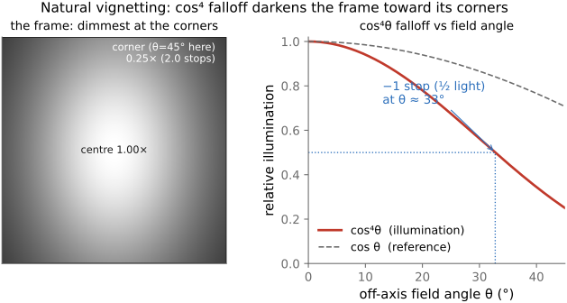
Off-axis ($\cos^4$) falloff. One prediction falls straight out of this irradiance integral. Rays reaching the corners of the frame arrive obliquely, so the same scene radiance delivers less irradiance there: the aperture-and-area geometry of the pixel integral works out to a $\cos^4\theta$ dimming toward the edges, called natural vignetting (Figure 2.8.3). It is distinct from optical vignetting — lens elements physically blocking edge rays, covered in Optics — in that natural vignetting is a clean consequence of the pixel-integral geometry alone.

2.8.3 Exposure values (EV) and stops🔗⧉

The pixel integral hands back a linear amount of light: double the aperture area or double the time and you double the number. Photographers almost never speak that way. They count light in stops, where one stop is a factor of two, because both the eye and the medium respond to ratios rather than differences (the same logarithmic story behind gamma encoding and Weber's law, Perceptual color and trichromatic vision). A stop is the natural quantum of exposure: one doubling, one halving, one bit of light. Written on the log$_2$ scale the integral lives on, the whole messy business of exposure becomes simple addition and subtraction.

The power of the unit is that it is the same unit on every axis of the integral. One stop of aperture (a $\sqrt2$ step in the f-number, since light goes as $1/N^2$, Lens image formation), one stop of shutter (a factor of two in time $t$), and one stop of ISO (a factor of two in gain) all change the brightness by the identical factor of two, so they are freely interchangeable. That commensurability is exactly what lets the three trade against one another, the exposure triangle: give back a stop of light on one leg, take it up on another, and the exposure is unchanged. Many different aperture-shutter-ISO combinations therefore land on the same brightness, a redundancy photographers call equivalent exposures and rely on constantly (the faucet-and-bucket reciprocity of Exposure).

To name a whole family of equivalent settings with a single number, photography uses the exposure value (EV):

the base-2 logarithm of the aperture-area-over-time ratio (at a reference ISO of 100). One EV is one stop. Every $(N, t)$ pair on the same EV describes the same exposure, so a single EV names an entire diagonal of the aperture-shutter grid:

Read across: each stop you close the aperture is paid back by one stop of slower shutter, and the exposure never moves. Because EV folds the settings into one number, it doubles as a measure of scene light. At ISO 100 the same EV names how bright the scene is (sometimes called the light value): a meter's reading, $L = K N^2/(t S)$, is EV in disguise, and the old sunny 16 rule ("bright sun is $f/16$ at 1/ISO") is nothing but a printed EV chart, one EV per lighting condition.

Once you have the unit, it turns up everywhere, which is the real reason to learn it. Meters report in EV, and every metered scene is placed on the EV ladder relative to mid-gray. Exposure compensation is dialed in EV ($+1$ EV to keep a snowfield white, $-1$ for a black cat), a direct nudge along the ladder. Auto-bracketing shoots frames at, say, $-2, 0, +2$ EV to merge into one high-dynamic-range image (HDR merging). A scene's dynamic range, a sensor's, a display's, are all quoted in stops (the ratio of brightest to darkest, in powers of two). Neutral-density filters are sold in stops (an ND8 is three stops), a lens's speed is "one stop faster," flash and studio lights meter in stops, and the noise story is a stop story too: because shot noise is set by photon count, every stop less light collected costs half the photons and a predictable step of signal-to-noise ratio (Noise). Stops and EV are the shared logarithmic language in which exposure, metering, dynamic range, filtration, and noise are all spoken; the full exposure and metering practice built on them is Exposure.

2.8.4 Splitting the integral🔗⧉

The integral we have just written is the bedrock of ordinary image formation: it projects a moving, three-dimensional world, seen through a finite lens, onto a flat two-dimensional image, collapsing aperture, area, wavelength and time into a single number per pixel. But a whole branch of computational photography refuses that collapse. Rather than integrate each axis away at capture, it slices and dices the integral — measuring an axis in pieces and reuniting them afterward — to recover the information the single integral throws out, and with it the freedom to form the image a posteriori.

Each axis can be split:

• Burst imaging splits the time integral into many short exposures, so they can be aligned before they are summed — recovering sharpness a single long exposure would have smeared, and putting motion blur under control after the shot (11 Multiple exposure imaging).
• Plenoptic / light-field cameras split the aperture integral, recording rays by the direction they came through the lens — so depth of field and focus can be chosen after the shot (14 Light fields and plenoptic cameras).
• Higher-resolution sensors split the spatial (pixel-area) integral, in the most mundane way on this list: more, smaller photosites, each averaging over a smaller footprint, so the box-filter narrows and finer detail survives the sampling (the sampling-and-antialiasing trade above). What looks exotic on the other axes is, on this one, just "more megapixels." Quad Bayer sensors make the split a choice taken after metering: the color-filter array groups photosites into $2\times2$ tiles that share one color, so in good light the four sub-pixels are remosaicked to full resolution (the integral split into four finer samples), while in dim light they are binned into one larger effective pixel (the integral quietly re-collapsed) for more light and less noise; staggering the exposures across the four even yields single-shot high dynamic range. The phone sensor that advertises "48 MP" yet hands you clean 12 MP files is doing exactly this: deciding, shot by shot, whether to split the spatial integral or simply perform it (Demosaicking).
• Hyperspectral imaging splits the wavelength integral into many narrow bands, replacing the three coarse color numbers with a full spectrum at every pixel.
• Polarization imaging splits a fifth axis: filters rotated to multiple angles separate light by polarization, giving a handle on specular highlights and reflections — cutting glare, or pulling a reflection apart from what sits behind the glass.

In every case the move is the same — don't integrate yet; record the pieces and decide later — and it is why so much of this book is about what becomes possible once the integral is no longer a foregone conclusion.

This completes the picture-forming side of measurement: a camera selects a slice of all the light in the world — the plenoptic function — and integrates it over aperture, area, wavelength, and time. The device that performs that integral physically — a grid of photosites counting photons, read out as numbers, and the shutter that times them — is the subject of the next chapter; the unavoidable jitter in the photon count, the noise it imposes, follows after that.