draft · v0.1.226
💬Comments welcome. To leave a note, select any text and click the note / highlight button that pops up — or open the panel with the tab at the top-right (‹). Notes are visible only inside our private review group.
Computational Photography, an AI-powered Slopendium — 02 Fundamentals
expand to📖 Full book outline1 parts · 17 chapters · 83 sections · 124 figures embedded · 12 placeholders · double-click a figure to enlarge
Part 2 FUNDAMENTALS OF IMAGING
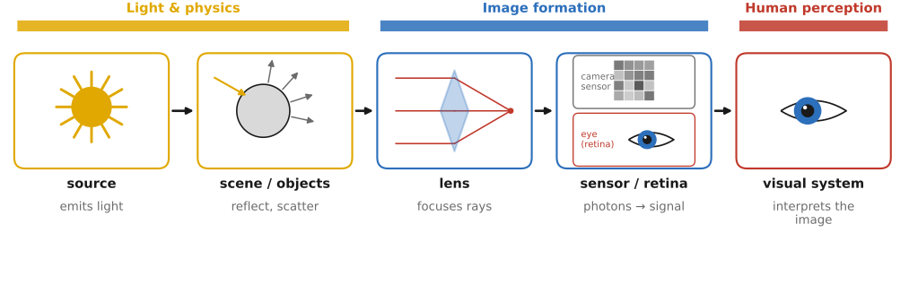
fig-light-journey
fig-light-journey · FUNDAMENTALS part opener — the journey of light: source → scene (reflection) → lens → sensor / retina → visual system, each step labelled with its chapter
**Photography means writing with light** — from the Greek *phōs* ("light") and *graphē* ("drawing"). This first part follows light on its entire journey and studies each step in turn.
• **the path of light** (and the chapters that follow it): a **source** emits light → it strikes **objects** and is reflected, absorbed, and scattered (the scene) → it passes through a **lens** → it lands on a camera **sensor** or the **retina**'s cones and rods → and the **visual system** interprets it.
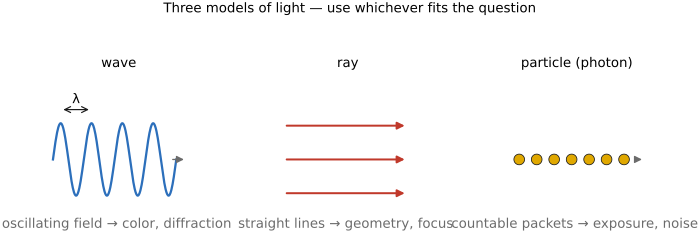
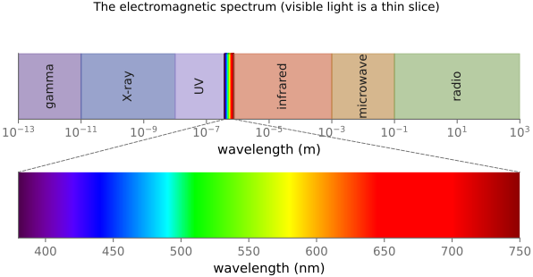
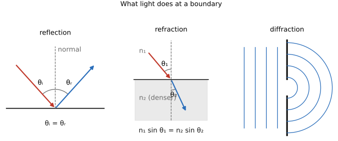
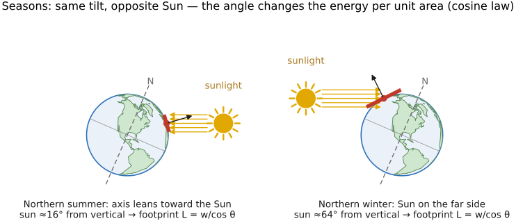
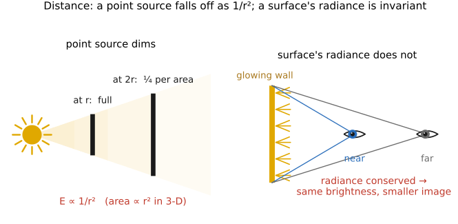
• **Light and physics** — what light *is* (wave / ray / photon), how it interacts with matter (reflection, refraction, scattering, the BRDF), and how we *measure* it (radiometry: radiance, irradiance, the inverse-square and cosine laws).
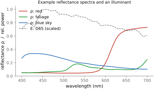
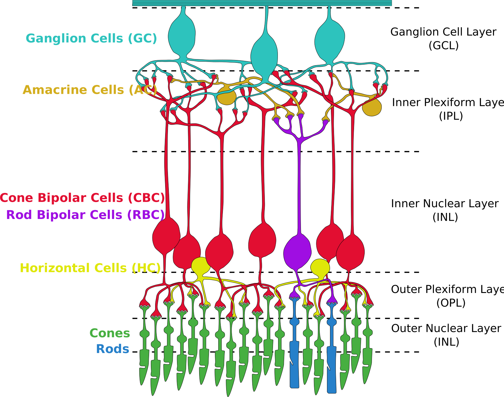
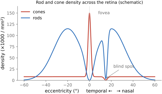
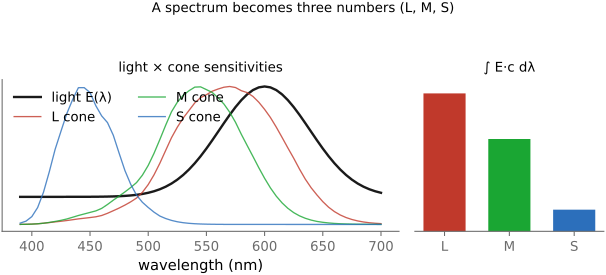
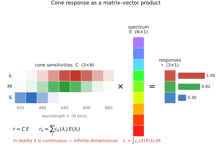
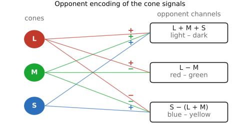
• **Human perception and color** — the eye and visual system; why three **cones** make us trichromatic; color as the projection of a spectrum onto three numbers; opponent processing, constancy, and the contrast sensitivity function. *(Placed early, right after light, because color is made in the observer and grounds everything downstream — encoding, white balance, JPEG, tone mapping.)*
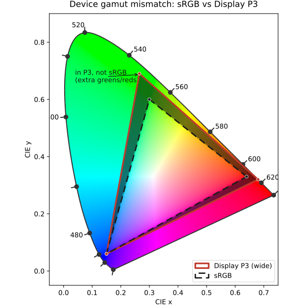
• **Measuring and encoding color** — the engineering payoff: **measuring** color (CIE), **encoding** it (linear / gamma / log, color spaces, CIELAB), and **reproducing** it (additive vs subtractive synthesis, gamuts, white balance, color management).
• **Image formation and linear perspective** — how a lens turns 3-D rays into a 2-D image (pinhole, perspective projection), depth of field, the **sensor** and the exposure triangle, **noise**, and the abstract framing the book leans on: imaging as a **linear system** and as an **inverse problem**.
• **The limits of the medium** — having built the camera and the image from physics, step back and ask what a picture fundamentally cannot do: it is flat, framed, single-viewpoint, static, and limited in contrast and gamut, while the world and the eye are none of these. (The camera as an instrument and the question of photographic objectivity move to the next part, [[Photography]].)
• **skippable, but foundational**: a reader who only wants to code can jump straight to BASIC IMAGE PROCESSING — but the **big lessons** of this part recur everywhere later. The ones to carry forward:
• **multiplicative vs additive** — much of imaging is *multiplicative* (illumination × albedo, contrast), some *additive* (incoherent light from different sources, blur); the right **encoding** (linear / log / gamma) follows from which one you are doing (→ [[Big Lessons]]).
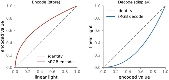
• **gamma / ratios matter** — perception is roughly logarithmic, so we store images **gamma-encoded** to spend code levels where the eye looks; what matters is *ratios*, not absolute values.
• **noise is affine** — sensor noise is **read + shot** (a constant plus a term that grows with the signal); because shot noise is **Poisson**, SNR is worst in the **shadows**, which is exactly where noise *looks* worst.
• **projective geometry is matrices + a division** — perspective projection is a **linear map in homogeneous coordinates** followed by a divide-by-depth; that single trick handles cameras, warps, and stereo.
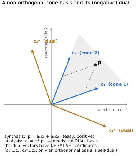
• **color is non-orthogonal and non-negative** — the cone "axes" overlap and light cannot be negative, which is what makes color sensing and reproduction genuinely hard (no perfect set of primaries; white balance is never exact).
• **by the end of this part** you can trace a photon from a lamp to a perceived color, reason quantitatively about exposure and noise, and you will carry the small set of principles the rest of the book keeps reusing.
2.1 Light and physics
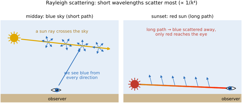
• chapter intro: a working model of light — its **color** (spectrum), its **interaction with surfaces**, and its **energy** (radiometry); closes with the **plenoptic function** that ties the pipeline together
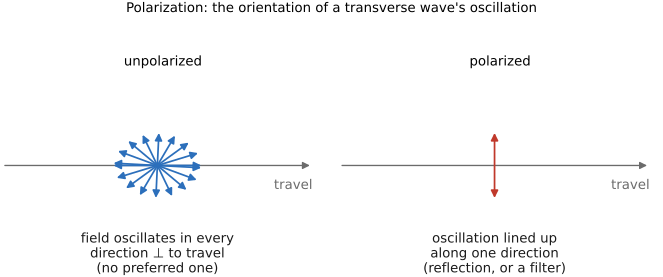
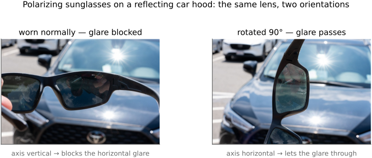
2.1.3 Polarization
2.2 Perceptual color and trichromatic vision
2.3 Human Vision
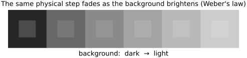
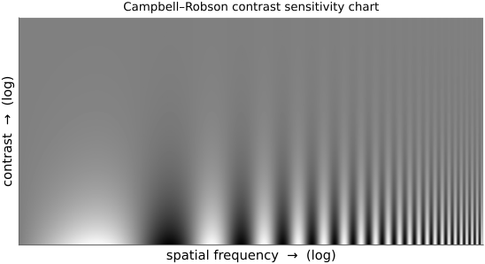
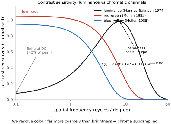
• the perceptual machinery the visual system runs *on top of* color: adapting to level, discounting the illuminant to report surface reflectance (constancy), working in ratios (contrast), and resolving detail unevenly across spatial/temporal frequency (the CSFs) — the properties compression, tone mapping, and display design optimize for.
2.4 Animal eyes
fig-eye-evolution
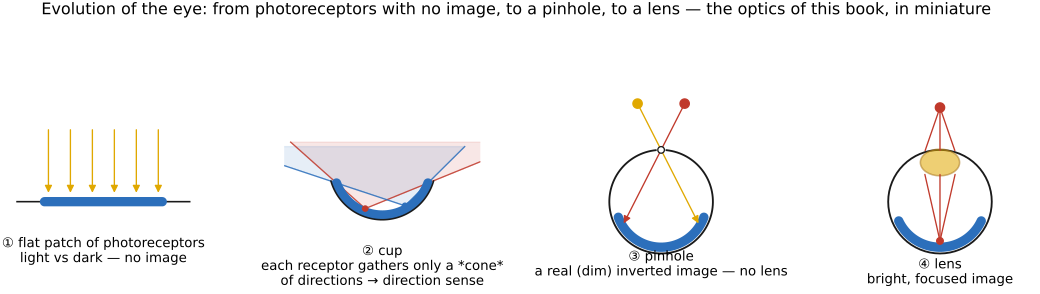
fig-eye-evolution · the evolution of the eye, in cross-sections: flat photoreceptor patch (no image) → cup (directional) → pinhole (an image, no lens) → lensed eye — recapitulating sensor → camera-obscura → lens (Bonus: animal eyes) 🟨
• **the eye evolved as a sequence of small improvements**, and it recapitulates the optics of this book — from "no image" to a focused one. Following Nilsson's stages (Land & Nilsson, *Animal Eyes*):
• **a flat patch of photoreceptors** (an *eyespot*): just **photosites**, **no image formation** — it tells light from dark and, crudely, which side has *more* light (phototaxis), but cannot form a picture. This is the bare **sensor** with no optics.
• **a concavity / cup**: fold the patch into a **pit** and the rim's shading gives **directional** sensitivity — the deeper the cup, the better you can tell *where* light comes from.
• **a pinhole**: close the cup almost shut → a **pinhole eye**, a real (if dim) **image** with no lens at all (the **nautilus** still uses one) — exactly the camera obscura of [[#Pinhole image formation and linear perspective]].
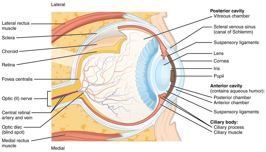
• **a lens**: fill the aperture with a **refractive lens** (often a graded-index sphere) → a **bright, focused** image, independently evolved in fish, cephalopods, and vertebrates. Add a **cornea, iris, and accommodation** and you have the human eye.
• so the human eye is *one* solution; evolution reached the same goal by very different routes (below).
• **a tour of those other solutions** — a useful contrast to the human eye and to camera design:
• **compound eyes** (insects): many **ommatidia** → wide field of view and fast temporal response, but low spatial resolution
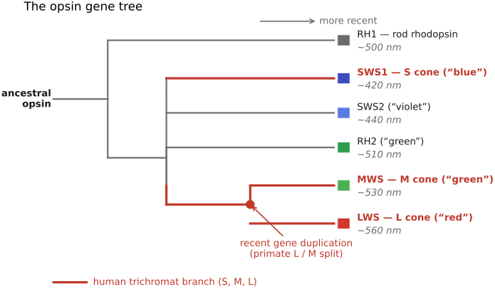
• **more cone types**: birds / reptiles are **tetrachromatic** (a 4th cone, into the UV); the **mantis shrimp** has ~12–16 photoreceptor classes (yet poor color *discrimination* — it seems to recognize rather than compare) — the **divergence of opsins** across animal groups is the color sidebar in [[#Color]]
• **tapetum lucidum** (cats, deer): a reflective layer behind the retina that boosts night vision (and causes eye-shine)
• **polarization vision** (cephalopods, many insects): they see light's **polarization** — a channel we're blind to
• **other eye designs**: **pinhole** (nautilus), **mirror eyes** (scallops — image formed by a concave mirror, not a lens), and the front-facing (**stereo**) vs side-facing (**field-of-view**) placement trade-off
• further reading: Land & Nilsson, *Animal Eyes*; the "Evolution of Eyes" chapter in *Vision* (Cambridge); a friendly overview at phos.co.uk, "The Evolution of Sight".
2.4.1 The optics: many ways to form an image
2.4.2 The color vision: opsins remixed
2.5 Measuring and encoding color
2.6 Pinhole image formation and linear perspective
fig-camera-obscura
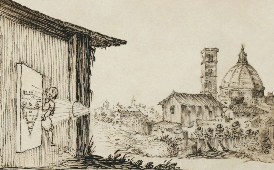
fig-camera-obscura · camera obscura / pinhole (artist's) 🟨
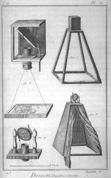
fig-camera-obscura-apparatus
fig-camera-obscura-apparatus · camera obscura apparatus (Diderot engraving) 🟨
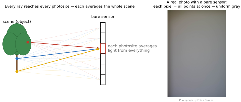
fig-bare-sensor-averaging
fig-bare-sensor-averaging · a bare sensor averages all rays 🟨
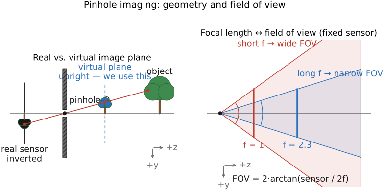
fig-pinhole-fov
fig-pinhole-fov · pinhole geometry: real (inverted) vs virtual (upright) image plane, and focal length → field of view 🟨
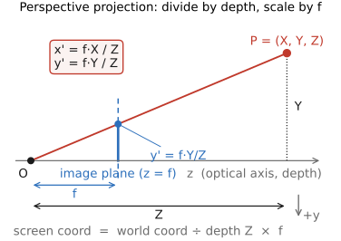
fig-perspective-projection
fig-perspective-projection · perspective projection equation: x'=f·X/Z, y'=f·Y/Z (divide by depth, scale by f) 🟨
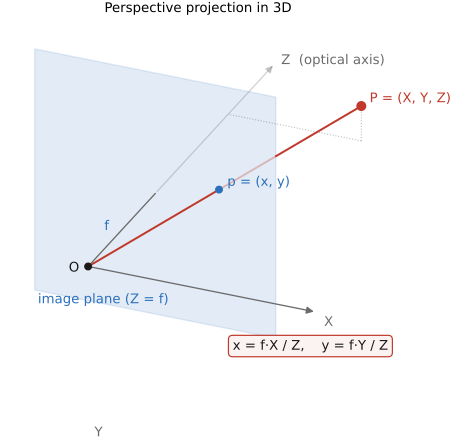
fig-perspective-projection-3d
fig-perspective-projection-3d · perspective projection in 3D: P=(X,Y,Z) → p=(x,y) on the image plane through the pinhole 🟨
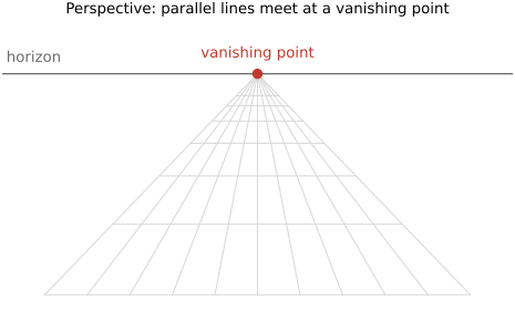
fig-perspective-vanishing-points
fig-perspective-vanishing-points · perspective projection + vanishing points 🟨
⬜ figure not yet created
focal length vs subject distance (background compression) fig-focal-length-compression
fig-face-distortion-sim
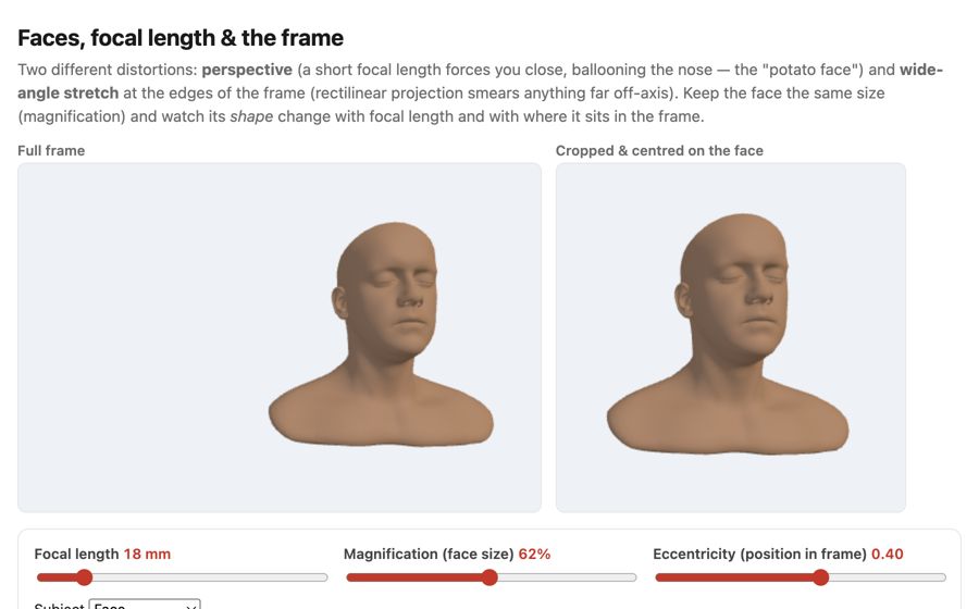
fig-face-distortion-sim · live face-distortion simulator (web edition): focal length + magnification + eccentricity controls with a full-frame view and a face-cropped view, showing the close-wide "big nose" perspective and the wide-angle edge stretch at constant face size; subject = a face, a grid sphere, or one of six diverse Meshy humans framed on the face; static fallback is a screenshot. *Human 3D models generated with Meshy AI.*
fig-dolly-zoom-sim
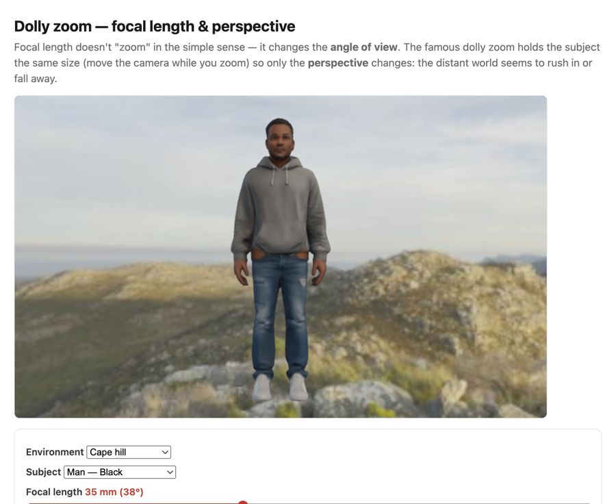
fig-dolly-zoom-sim · live dolly-zoom simulator (web edition): hold the subject size while focal length and camera distance trade off so only perspective / background scale changes; log focal (12–200 mm) + distance sliders, realistic Poly Haven environments, subject = head bust or one of six diverse Meshy humans. *Human 3D models generated with Meshy AI.*
fig-portrait-lighting-sim
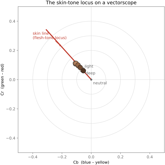
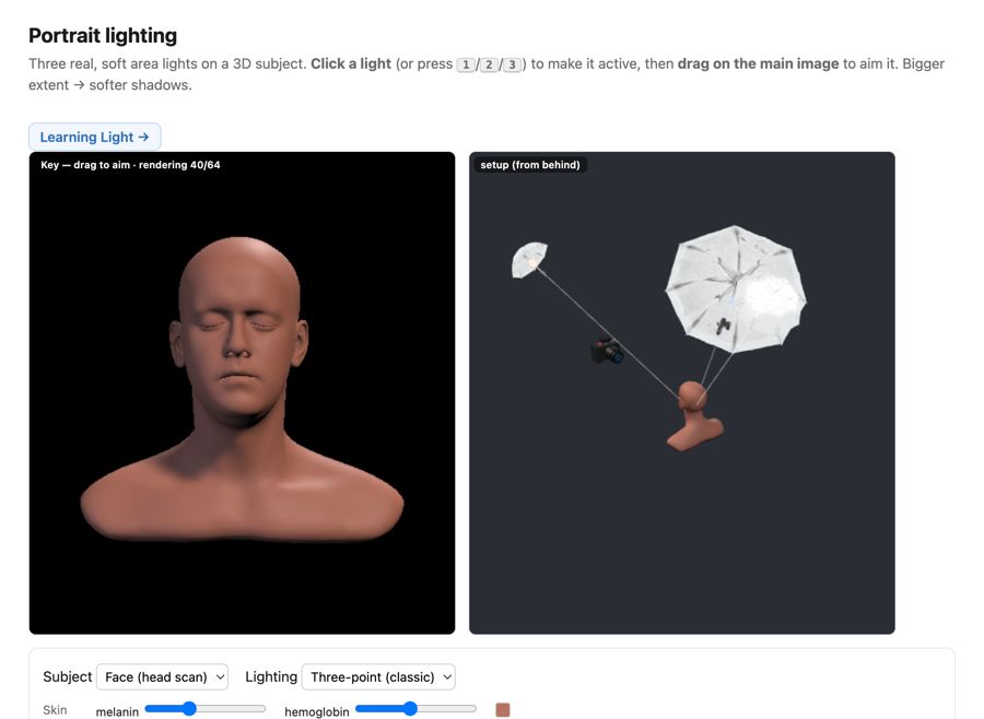
fig-portrait-lighting-sim · live portrait-lighting simulator (web edition): three soft area lights (key/fill/kicker — az/el/extent/intensity/colour, area-light-supersampled soft shadows) on a 3D face with a physiological melanin/hemoglobin skin model; a from-behind setup view with Meshy studio umbrellas + a camera rig; lighting presets; static fallback is a screenshot. *3D umbrella generated with Meshy AI.*
fig-keystoning-cause
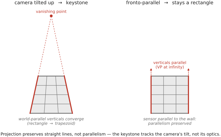
fig-keystoning-cause · keystoning is the tilt, not the lens — a camera tilted up makes world-parallel verticals converge (façade → trapezoid), while the fronto-parallel shot keeps them parallel; projection preserves lines, not parallelism 🟨
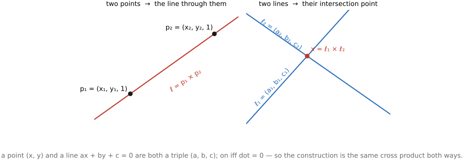
fig-point-line-duality
fig-point-line-duality · point↔line duality in homogeneous 2D: two points → a line, two lines → a point (same cross product) 🟨
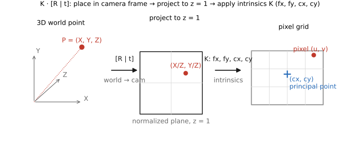
fig-projection-decomposition
fig-projection-decomposition · projection-matrix decomposition K·[R matplotlib, 3-stage pipeline
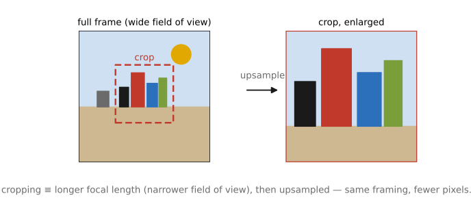
fig-crop-focal-length
fig-crop-focal-length · cropping = changing focal length: full frame vs a crop box ≡ a longer-focal-length capture, upsampled 🟨
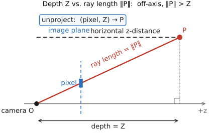
fig-depth-vs-ray-length
fig-depth-vs-ray-length · depth (z coordinate) vs ray length ‖P‖ from camera to a 3D point; unproject (pixel + depth → 3D) 🟨
• sensor alone would capture a diffuse light. We need to select which rays from which part of the scene contribute to which pixel.
equations
pinhole projection x = f·X/Z, y = f·Y/Z
homogeneous p ≈ K·[R|t]·P
field of view = 2·arctan(sensor / 2f)
2.6.3 Camera in a general configuration
2.6.7 Wide-angle distortion: spheres bulge and faces stretch at the edges
2.7 Lens image formation
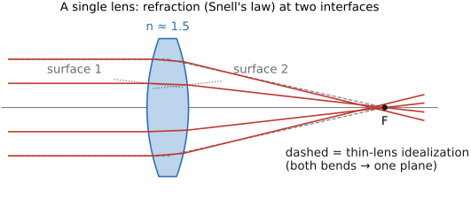
• chapter intro: from the **pinhole** (sharp but dim) to a **lens** (bright but with one focus plane) — refraction at curved surfaces, the thin-lens linearization, and the depth-of-field that the finite aperture forces on us
2.8 Image measurements as integrals
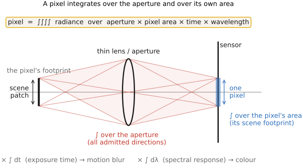
• chapter intro: the unifying idea behind sensing — **measurement = integrating a slice of the plenoptic function** — then the physical sensor that does it (photosites, CCD/CMOS) and the **noise** that limits it
• sidebar — **photography as objective measurement**: the medium's long arc bends toward objective measurement (film/print = a *performance*; → measurement). The **digital sensor** is the far end: because each photosite *counts photons*, a **raw** image is ≈ a **calibrated radiometric measurement** — a physical map of scene radiance, in real units, of one snapshot of time — not just a rendering. This is what makes HDR / depth / deblur possible: the pixel numbers must *mean* something physical. Ties to the intro's **generation → measurement → generation** arc (→ [[01 Intro]]).
2.8.3 Splitting the integral
2.9 Depth of field
fig-circle-of-confusion
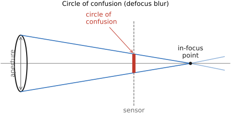
fig-circle-of-confusion · finite aperture & circle of confusion
fig-defocus-vs-parameters
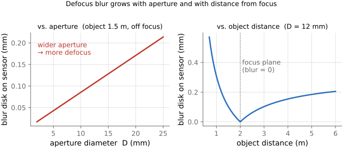
fig-defocus-vs-parameters · defocus blur (CoC) vs aperture and object distance 🟨
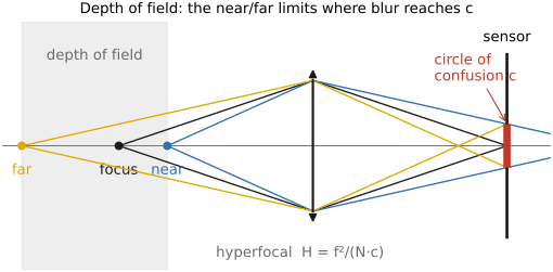
fig-depth-of-field
fig-depth-of-field · near/far limits where blur reaches c (linearized DoF) 🟨
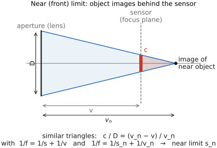
fig-dof-derivation-near
fig-dof-derivation-near · near (front) limit by similar triangles — all quantities 🟨
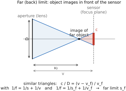
fig-dof-derivation-far
fig-dof-derivation-far · far (back) limit by similar triangles — all quantities 🟨
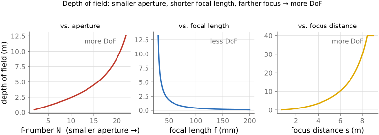
fig-dof-vs-parameters
fig-dof-vs-parameters · DoF vs aperture, focal length, focus distance 🟨
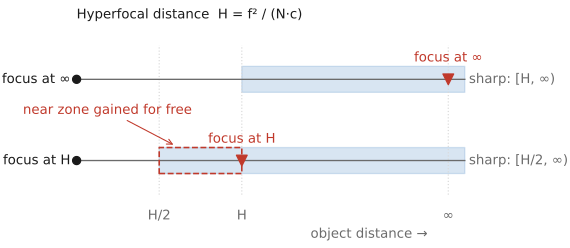
fig-hyperfocal
fig-hyperfocal · hyperfocal: focus at H → sharp from H/2 to ∞ 🟨
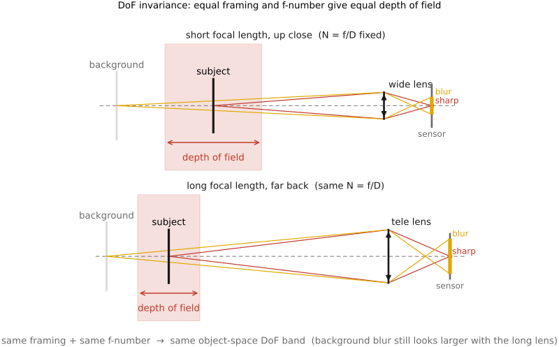
fig-dof-same-framing
fig-dof-same-framing · same framing + same f-number → same object-space DoF (short vs long focal length); background blur still looks larger with the long lens 🟨
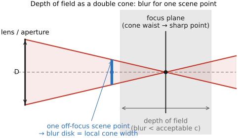
fig-dof-double-cone
fig-dof-double-cone · object-space DoF as a double cone in front of the lens, waist on the focus plane (the blur for one scene point) 🟨
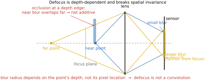
fig-dof-depth-dependent
fig-dof-depth-dependent · defocus is NOT a convolution: blur radius depends on scene depth (not pixel location), and occlusion at depth edges 🟨
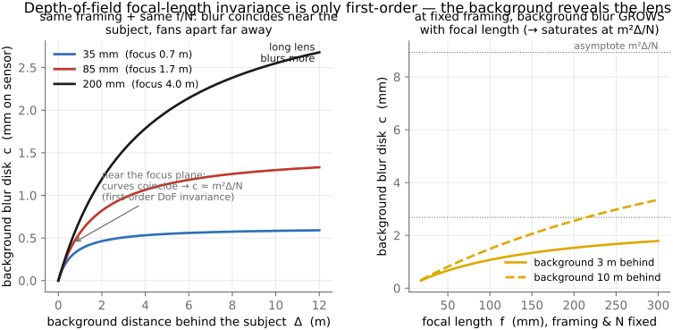
fig-dof-background-blur
fig-dof-background-blur · DoF focal-length invariance is only first-order: background blur c vs background distance for 35/85/200 mm (matched framing & N) coincide near the subject and fan apart far away; + c vs focal length showing growth/saturation
• **defocus / circle of confusion**: a point off the focus plane images to a point that is not on the sensor, so the aperture cone meets the sensor as a blur disk — the **circle of confusion**. A point still counts as sharp while its disk stays within an acceptable c. [CoC figure]
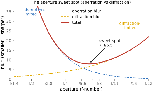
• the blur disk grows with the **aperture** (wider → bigger disk) and with the **object's distance from the focus plane** (zero exactly at focus); focal length and focus distance enter too. [defocus-vs-parameters figure]
• **depth of field** = the *range* of object distances whose blur disk stays within c; the **near** and **far** limits are where the blur just reaches c. [DoF near/far figure — each cone carried out to the CoC at the sensor]
• **deriving the limits**: on the image side a near-limit object images *behind* the sensor and a far-limit object *in front* of it; **similar triangles** relate the aperture D, that convergence distance, and the circle of confusion c — and together with the conjugate relations (1/f = 1/s + 1/v) they fix the near (front) and far (back) object-distance limits. [near-limit and far-limit similar-triangle figures]
• **hyperfocal distance** H = f²/(N·c): focus there and everything from **H/2 to infinity** is acceptably sharp — the focus setting that maximizes DoF (focusing at ∞ instead wastes the H/2…H zone). [hyperfocal figure]
• DoF **grows** with a smaller aperture (larger N), a shorter focal length, and a greater focus distance — these are the paraxial (linearized) formulas; the accurate model is in the Optics part. [DoF-vs-parameters figure]
• **the surprising invariance** (the lecture's flagged "important conclusion"): for a **fixed framing** (same subject size) and a **fixed f-number**, the depth of field in **object space** is essentially **independent of focal length** — switching 28 mm → 100 mm forces you to step back, and the larger physical aperture cancels the longer focal length. So "long lenses have shallow DoF" is really about **magnification**, not focal length per se. (The *background* still looks more blurred with the long lens — that's magnification of the out-of-focus disk, not a DoF change.) [same-framing/same-N → same DoF figure]
• ⚠️ **but the invariance is only *first-order* — the background gives the focal length away.** "Same framing + same f-number → same DoF" is the **small-defocus (paraxial)** result: it holds for the **near/far acceptable-sharpness limits straddling the subject**, but **not** for how hard a *distant* background is thrown out of focus. **Derivation** (thin lens; blur-disk diameter on the sensor): a point at distance $s_b$, with the lens focused at $s_f$, images to a circle of confusion $c \approx \dfrac{f^2}{N}\,\dfrac{|s_b-s_f|}{s_b\,s_f}$. **Fix the framing** — subject magnification $m=f/s_f$ held constant, so $s_f=f/m$ — and **fix $N$**, with the background a gap $\Delta=s_b-s_f$ behind the subject:
$$c(f)=\frac{m^2\Delta/N}{\,1+ m\Delta/f\,}\ \xrightarrow[f\to\infty]{}\ \frac{m^2\Delta}{N}.$$
The subject-zone DoF is ~independent of $f$ (the leading $f$ cancels — the **first-order invariance**), but the **background blur grows monotonically with focal length**, saturating at $m^2\Delta/N$. Two shots matched in framing *and* aperture render the **subject** identically, yet a **200 mm melts a far background far more** than a 35 mm: the correction term is order $m\Delta/f$ — negligible for a background near the focus plane (invariance looks exact), but dominant once the background is many focus-distances away. This is exactly why portrait shooters reach for long lenses for "background separation" even though the DoF on the *face* is unchanged. **Full derivation + plots** of $c$ vs. background distance for 35 / 85 / 200 mm (fixed framing & $N$) — the curves coincide near the focus plane and fan apart far from it. [`fig-dof-background-blur`]
• **object-space picture & a caveat**: the simplest view is a **double cone** in front of the lens whose waist sits on the focus plane — it gives the blur for **one** scene point. But **defocus is *not* a spatially-invariant convolution**: the circle of confusion depends on each point's **scene depth** (not its pixel location), and at depth discontinuities **occlusion** matters — which is why naive "just blur the image" fakes look wrong, and why light-field / depth-aware methods (Advanced) do better. [object-space double cone; depth-dependent-blur + occlusion figure]
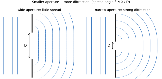
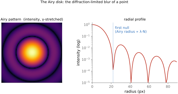
• **sensor size scales DoF**: shrink the sensor (keeping FOV) and both the circle of confusion and the aperture shrink, so DoF grows **linearly** with sensor size — why phone cameras have huge DoF (and resort to *computational* background blur), and why **macro is easier on small sensors** (a scaled-down camera photographs a scaled-down world — modulo diffraction)
• 🖱️ **Interactive (web edition):** a live **macro depth-of-field simulator** — a to-scale thin-lens diagram, a lens-supersampled 3D photo (real bokeh), and a circle-of-confusion-vs-distance plot all driven by one shared optics model (focal length, f-number, sensor, focus distance, subject–background gap). A 3D bug (beetle / bee / ladybug) over a flower makes the macro lesson vivid: focus lands on the front of the face and the rest of the body, antennae, and background all fall out of focus. [fig-depth-of-field-sim; interactive] *(bug & flower 3D models generated with Meshy AI — acknowledge in the caption)*
equations
acceptable blur = circle of confusion c
defocus blur diameter b = D·|v − v′|/v′
hyperfocal H = f²/(N·c)
near limit D_n = s(H−f)/(H+s−2f)
far limit D_f = s(H−f)/(H−s)
total DoF = D_f − D_n
2.10 Motion blur
• **blur from subject motion**: $b_{px}\approx f_{px}\,v\Delta t/D$ — a straight streak = image velocity × exposure (constant-velocity linearization); only cross-axis motion blurs
• **blur from camera shake**: translation $b\approx f_{px}\Delta_c/D$ (depth-dependent); rotation yaw/pitch $b\approx f_{px}\theta$ (**depth-independent**, small-angle); roll = spin about centre, grows with radius
• **which dominates**: ratio $\theta D/\Delta_c$ → rotation wins at normal distance, translation only up close (macro); rotation blur is **spatially non-uniform** so one kernel can't undo it (Whyte); IMUs measure the rotation to deblur (Joshi)
• **hand-holding rule** $\Delta t\lesssim 1/f$ s (×crop; ~2× faster for dense sensors); **image stabilization** cancels camera *rotation* (buys 3–5 stops) but not *subject* motion
• 🖱️ **Interactive:** motion-blur calculator — 3-D scene (Meshy walking human / car), temporal-supersampled blur, world+screen readout by source, motion-vector & flow-colour overlays, hover pixel scale [fig-motion-blur-calculator; interactive]
2.11 Sensors: photosites, CCD vs CMOS
fig-sensor-microlens
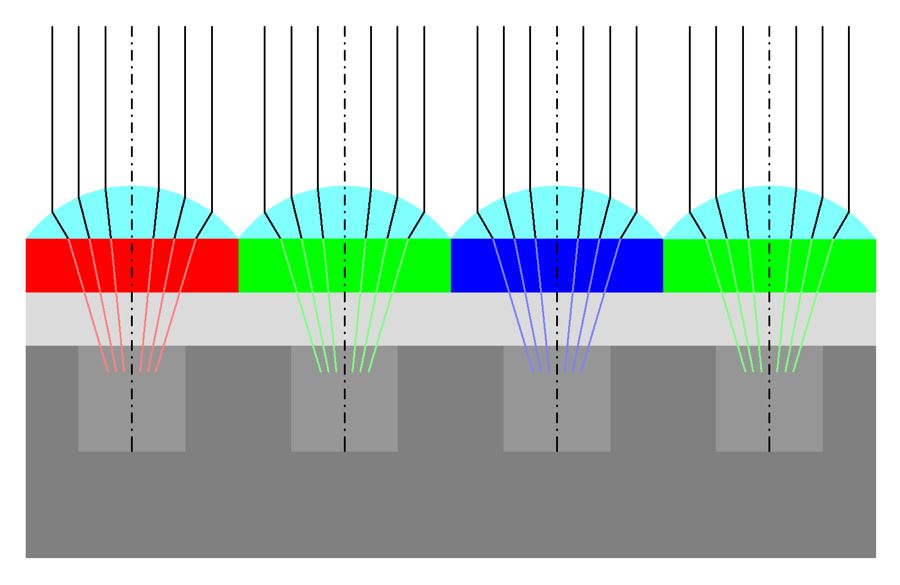
fig-sensor-microlens · sensor cross-section: microlens → filter → photosite 🟨
⬜ figure not yet created
CCD bucket-brigade readout vs CMOS read-in-place schematic fig-ccd-vs-cmos
fig-slowmo-axis
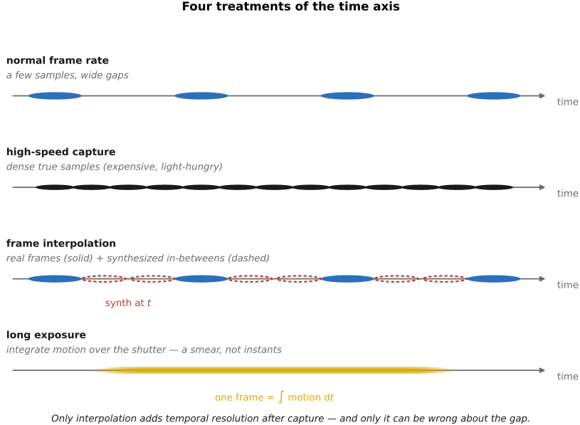
fig-slowmo-axis · four ways to treat the time axis on a shared timeline — normal capture (sparse), high-speed (dense true samples), interpolation (sparse reals with synthesized in-betweens), and long-exposure blur (the integral); only interpolation adds resolution after capture and can be wrong 🟨
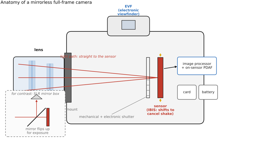
fig-mirrorless-anatomy
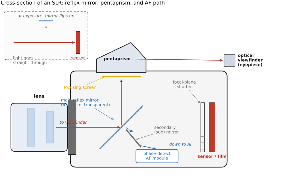
fig-mirrorless-anatomy · labeled cutaway of a mirrorless full-frame camera (lens+mount, sensor/IBIS, mech+electronic shutter, EVF, processor/on-sensor PDAF, card+battery); SLR mirror-box inset for contrast
fig-rolling-shutter
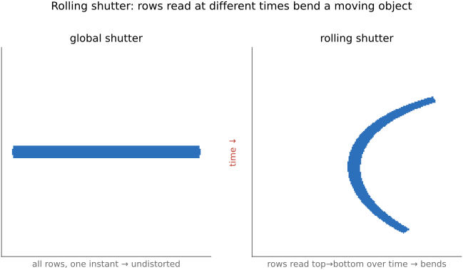
fig-rolling-shutter ·
fig-flash-sync
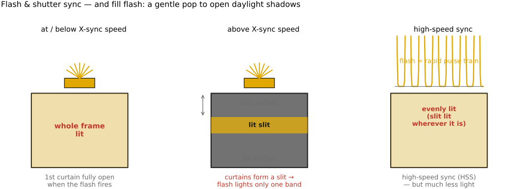
fig-flash-sync · flash & focal-plane-shutter sync: whole frame ≤ X-sync · slit/partial frame above it · high-speed-sync pulse train; fill-flash noted
fig-lippmann
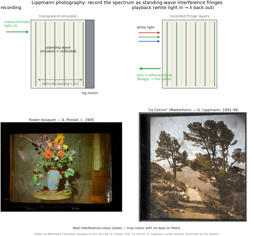
fig-lippmann · Lippmann interference colour photography: recording (standing wave in a mercury-backed emulsion, antinodes λ/2 apart) + playback (Bragg reflection of the original wavelength under white light)
2.11.3 Analog-to-digital conversion
2.11.6 Shutters
2.11.10 The impact of sensor size
2.11.11 How far sensors have come
2.12 Sensing color: multiplexing strategies
fig-color-multiplexing
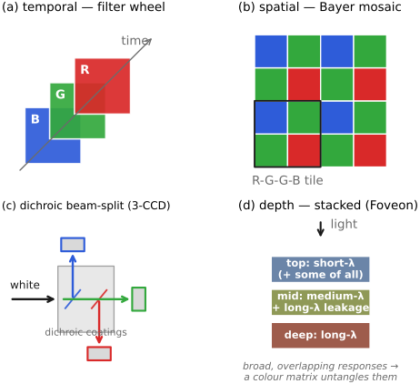
fig-color-multiplexing · four colour-sensing multiplexing strategies: temporal, spatial (Bayer), **dichroic 3-CCD** beam-split, depth (Foveon, with realistic broad/overlapping layer colours + colour-matrix note) 🟨
⬜ figure not yet created
temporal multiplexing artifact — Prokudin-Gorskii color fringes on moving water fig-prokudin-gorskii
• four ways to turn a monochrome sensor into a color one — **multiplex** the three (or more) measurements across some axis:
• **in time**: shoot R, G, B frames sequentially through filters — Maxwell's first color photograph (1861), **Prokudin-Gorskii**, flatbed scanners, astronomy filter wheels. Cheap and full-resolution, but **fails on motion** (the classic color fringes on moving water).
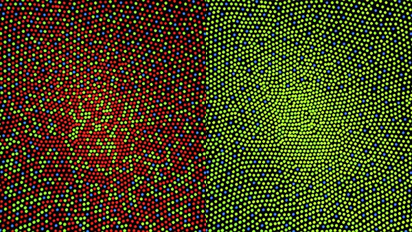
• **in space (the dominant choice)**: a **color filter array (CFA)** — the **Bayer mosaic** (2 green : 1 red : 1 blue) — one color per photosite, then **demosaick** to fill the rest; the eye does the same with its interleaved cone mosaic. Variants: Fuji's **X-Trans** (a larger, less-periodic tile to fight moiré) and **complementary CMY/CYGM** CFAs (more light through, messier color). Needs an **optical anti-aliasing (low-pass) filter** to tame high-frequency color artifacts, and suffers some channel **crosstalk**.
• **beam-splitter (prism)**: a **dichroic prism** splits the rays onto **three sensors** — **3-CCD / 3-chip**, the classic **broadcast video camera** — wasting no photons at full per-channel resolution, but bulky, costly, and hard to align.
• **in depth (stacked)**: stack wavelength-selective layers so one location senses all three — **Foveon** (silicon absorbs longer wavelengths deeper; used in **Sigma** cameras), echoing **Kodachrome**'s stacked dye layers. Full color at every pixel (**no demosaicking**), but trickier color separation and more chroma noise.
• **spectral / Lippmann**: record the standing-wave **interference** of the full spectrum (Lippmann, 1908 Nobel; a precursor to holography) — true spectral capture, not just 3 numbers.
• **hybrid**: combine these (e.g. spatial + temporal in video).
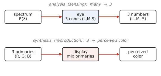
• this is *analysis* (sensing color) — the mirror of color *synthesis* (reproduction, above); the **demosaicking** algorithm itself is deferred to Basic Image Processing (which is why this is just the *sensing* half)
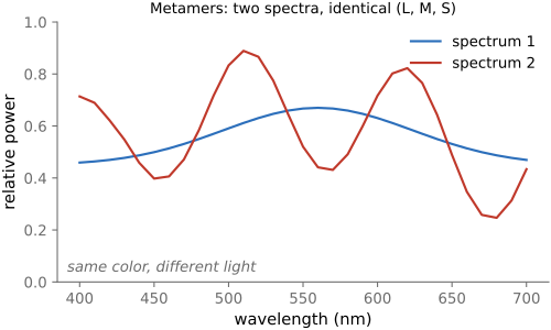
• **trichromatic (perceptual) vs spectral (physical) capture**: almost all imaging systems aim to capture **perceptual, trichromatic color** — three numbers that reproduce what a *human* would see (RGB ≈ the cones), so metamers are, by design, indistinguishable. **Multispectral / hyperspectral** imaging instead samples the **physical spectrum** in many narrow bands (tens to hundreds), keeping distinctions the eye throws away — for remote sensing, agriculture, art conservation, and machine vision, where the *material*, not the *appearance*, is what matters (and metamers must be told apart). Lippmann (above) is the limiting case: the full continuous spectrum.
2.13 Noise, signal-to-noise ratio and dynamic range
⬜ figure not yet created
noisy image + flat-patch histogram (ISO 3200) fig-noise-histogram
⬜ figure not yet created
noise vs ISO fig-noise-vs-iso
fig-noise-affine
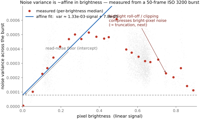
fig-noise-affine · measured noise variance is affine in brightness (σ²≈gain·I+read²) — real per-pixel variance vs mean from a 50-frame aligned ISO-3200 burst, with the affine fit, read-noise floor, and highlight roll-off (Noise, SNR, dynamic range)
fig-noise-gaussian-pixels
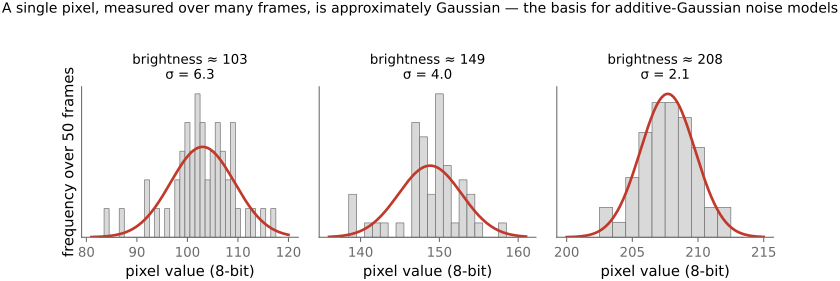
fig-noise-gaussian-pixels · a single pixel's value across many frames is ≈ Gaussian — per-pixel histograms from the ISO-3200 burst with Gaussian overlays (Noise)
fig-noise-truncation
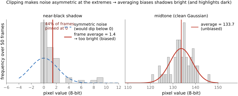
fig-noise-truncation · noise clips at black/white so it is not zero-mean at the extremes — a near-black pixel pinned at 0 ~44% of frames, its average biased bright, vs an unbiased midtone (Noise; denoising trap)
fig-snr-vs-stddev
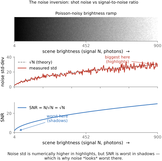
fig-snr-vs-stddev · noise std-dev map vs SNR map of a brightness ramp: std rises with brightness (∝√N), but SNR=√N is worst in the shadows 🟨
⬜ figure not yet created
**underexposure recovery — full-frame vs phone**: the same underexposed scene pushed up several stops in software, the full-frame frame cleaning up while the phone reveals amplified shadow noise / banding [fig-underexposure-recovery-ff-vs-phone fig-underexposure-recovery-ff-vs-phone
fig-results-montage
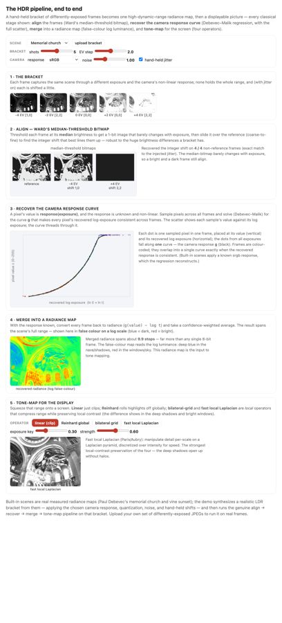
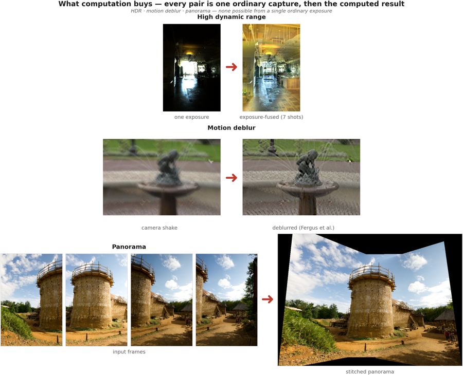
fig-results-montage · a montage of computational-photography results — HDR tone mapping, refocus-after-capture, motion deblur, a stitched panorama — the "look what computation buys you" opener
fig-dynamic-range-comparison
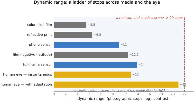
fig-dynamic-range-comparison · dynamic-range ladder in **stops** (horizontal bars): colour slide (~5–6) · reflective print (~6–7) · film negative (~12–13) · phone sensor (~10–12) · full-frame sensor (~14) · human eye instantaneous (~10–14) vs adapted (~20+) · an animal example · a typical sun-and-shadow scene (>20) — shows why no single capture holds a high-contrast scene (→ HDR)
⬜ figure not yet created
an animal or two
• the noise **sources** (their variances add):
• **photon / shot noise** — the Poisson statistics of *counting photons*: variance = mean, so σ = √N. Fundamental (it's the light itself), dominates the midtones/highlights; averaging N independent frames cuts it by √N.
• **read noise** — added by the amplifier / ADC on readout; signal-independent, dominates the **shadows** and sets the noise floor (hence dynamic range).
• **thermal / dark current** — electrons freed by heat, independent of light; grows with exposure time and temperature (long exposures & astrophotography → sensor cooling, dark-frame subtraction).
• **fixed-pattern / pattern noise** — per-pixel gain/offset non-uniformity (PRNU/DSNU), hot/stuck pixels, banding; *structured*, so it reads as worse than random noise of equal magnitude, and is removed by calibration (flat / dark fields).
• 💡 **Big lesson — in a *linear* image, noise variance is an *affine* function of brightness.** The variances add: shot noise gives a term **proportional to the signal** (Poisson, variance = mean, scaled by the gain) and read noise a **constant** floor, so the total is **variance ≈ gain·signal + read²** — a straight line in brightness. You can *measure* it: take an aligned **burst** of a static scene and, per pixel, plot the variance across frames against the mean — the points trace that line, slope = photon gain, intercept = the read-noise floor. And a single pixel's value over many frames is **≈ Gaussian**, which is what licenses additive-Gaussian noise models. [`fig-noise-affine` — per-pixel variance vs brightness, measured from a 50-frame ISO-3200 burst; `fig-noise-gaussian-pixels` — per-pixel histograms] → register [[Big Lessons]]
• 💡 **Big lesson — noise is *clipped* at black and white, so near the extremes it is *not* zero-mean.** A recorded value is clamped to [0, max]: near black the negative half of the noise is cut off (frames pile up at 0), near white the positive half is. So at the extremes the noise distribution is **asymmetric** and its mean is pushed **inward**. The consequence for **denoising**: any naive average/smoothing returns that biased mean, so it makes **shadows come out too bright and highlights too dark** — a bias every denoiser has to correct for (carried forward to [[#Denoising basics]] in BASIC). [`fig-noise-truncation` — a near-black pixel pinned at 0 a third of the time, its average biased bright; from the ISO-3200 burst] → register [[Big Lessons]]
• **the key intuition — it's about ratios (SNR)**: shot noise is **Poisson**, so σ = √N grows with brightness — measured noise is actually **higher in the highlights**. Yet noise *looks* worst in the **shadows**, because perception cares about the **signal-to-noise ratio** SNR = N/√N = √N, which is worst where N is small. "Ratios are all that matters" — the same reason we encode in gamma/log, and the motivation for ETTR (below — Photography 101). [std-dev map vs SNR map figure]
• **dynamic range** = the brightest recordable signal (sensor **saturation / full-well**) ÷ the **noise floor** (read noise in the shadows); it sets how much of a high-contrast scene fits in a *single* exposure → the motivation for **HDR** (Multiple exposure)
• **HDR (high dynamic range)**, sometimes called **wide dynamic range (WDR)**, is a deliberately **fuzzy** term — flag this. It gets used for at least four different things: the *scene* (a high-contrast world), the *capture* (multi-exposure / a high-DR sensor), the *file/encoding* (float or ≥10-bit radiance, e.g. OpenEXR, HDR10), and the *display* (an HDR monitor) — and, loosely, for the **tone-mapped "HDR look."** There is no single sharp definition; say which sense you mean. (Developed in [[Multiple exposure imaging]].)
• 💡 **Big lesson (L2.48) — dynamic range is set by full-well capacity over the noise floor**: a single exposure records from a **top** (the photosite's **full-well capacity** — where it clips to white) down to a **bottom** (the **noise floor** — read noise in the shadows); their **ratio is the dynamic range** (quoted in stops). You **widen** it with a **bigger well** (larger photosites — why a full-frame sensor out-ranges a phone) or a **lower floor** (cooling, lower read noise), and you **beat** it altogether by merging **multiple exposures** (HDR). The capture-side companion to **L2.49**: what bounds a shot is this *range*, not the bit depth. → register [[Big Lessons]]
• **examples, in stops** (the figure): a color **slide** is narrow (~5–6 stops), a reflective **print** ~6–7, **film negative** wide (~12–13 latitude), a **phone** sensor ~10–12, a **full-frame** sensor ~14; the **human eye** is ~10–14 stops *instantaneously* but ~**20+** once **adaptation** is allowed — and some **animals** do better in their niche; an outdoor sun-and-shadow scene can exceed **20 stops**, which is why no single capture holds it [fig-dynamic-range-comparison]
• **see it — recover an underexposed shot, full-frame vs phone**: shoot the *same* underexposed scene as **raw** on a **full-frame** camera and on a **phone**, then **push the exposure up** in software (e.g. +3–4 stops). The full-frame frame cleans up (deep full-well + low read-noise floor → wide dynamic range), while the phone frame breaks down into **shadow noise and banding** as the lift amplifies its read-noise floor — a direct, visible demonstration that **dynamic range scales with photosite / sensor size**, and exactly why phones lean on **burst / HDR+** (Multiple exposure) rather than a single exposure. [fig-underexposure-recovery-ff-vs-phone; photo — paired Fredo full-frame DNG + phone raw] *(also a coding exercise — see [[Exercises & Experiments]])*
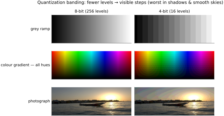
• 💡 **Big lesson (L2.49) — quantization is rarely the real problem**: with enough bits and a sane encoding, it's **noise and dynamic range** (this section) that bite — not the number of levels. The one exception is **gamma / banding in shadows**, which is exactly why gamma encoding exists (allocate codes perceptually); so "rarely" ≠ "never". Reminded again in BASIC → Image representation → *Float vs 8-bit*.
equations
shot noise Poisson (variance = mean), σ ∝ √N, SNR = √N
variances add (shot + read + thermal)
averaging N frames → noise /√N
PSNR = 10·log₁₀(MAX²/MSE)
dynamic range = full-well ÷ read-noise floor
2.13.1 Noise sources
2.13.2 The algebra of noise
2.13.3 Signal-to-noise ratio: it's about ratios
2.13.4 Dynamic range
2.13.5 Regimes, and how close we are to the limits
2.14 Imaging as a linear system
2.15 Imaging as an inverse problem
2.16 Limitations of the medium
2.17 Displays
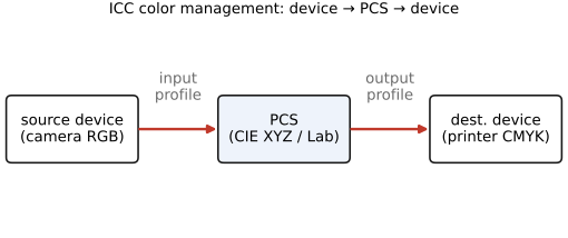
• chapter intro: the last link in the chain. The range of displays (phone, laptop, TV, projector, print) and how their characteristics — size and viewing distance, resolution, dynamic range, gamut, and viewing environment — shape both the experience and the processing. This chapter also carries color management: the ICC workflow and the industry standards that keep color consistent across capture, editing, and display. Forward-reference to [[Integral and immersive imaging]] for near-eye and immersive displays.