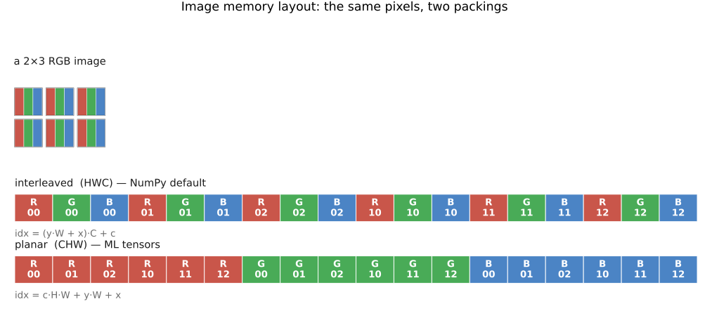
fig-image-memory-layout · a 2×3 RGB image packed into 1-D memory two ways — interleaved HWC (NumPy) vs planar CHW (ML), with the stride formulas (Image representation, BASIC) 🟨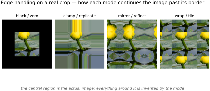
fig-edge-handling-photo · the four edge modes on a real crop — black / clamp / mirror / wrap continued past the border; real-image companion to `fig-edge-handling` (Image representation → falling off the edge, BASIC) ✅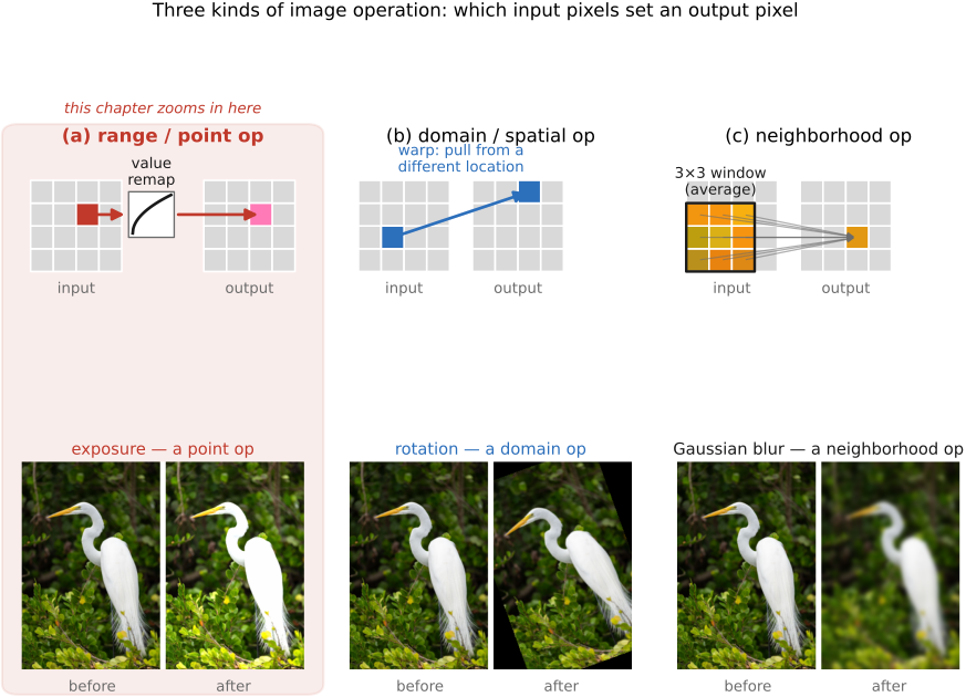
fig-operation-types · the three image-operation types — range (point) vs domain (spatial) vs neighborhood (Values / point ops, BASIC) 🟨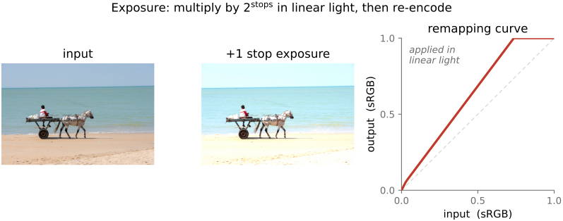
fig-point-op-exposure · exposure as a multiply in linear light: input, output (+1 stop), and the remapping curve (Basic Image Processing → point operations) 🟨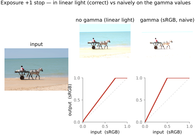
fig-point-op-exposure-spaces · exposure +1 stop done right (linear light) vs naively on the gamma values (over-brightens, clips at input ½): two outputs + remapping curves 🟨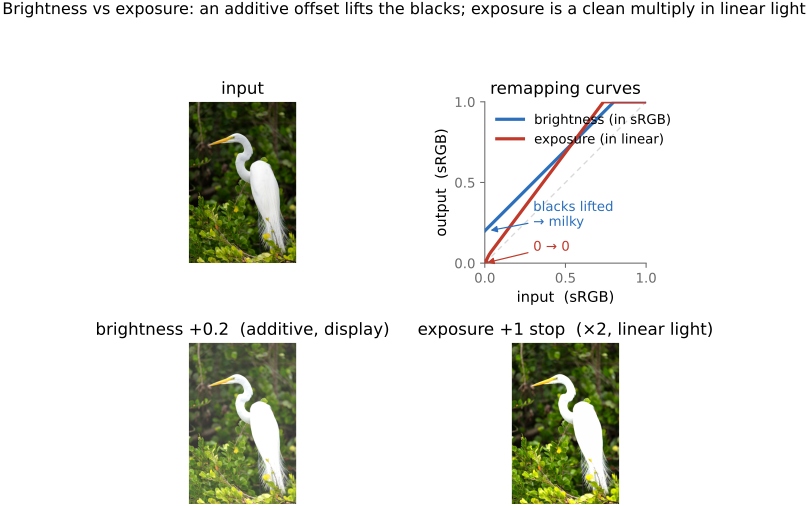
fig-point-op-brightness-vs-exposure · brightness (additive, lifts blacks → milky) vs exposure (×2 in linear light, keeps 0→0): two outputs + both remapping curves 🟨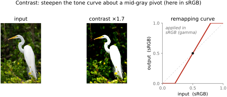
fig-point-op-contrast · contrast as a steeper tone curve about a mid-gray pivot: input, output, and the remapping curve (Basic Image Processing → point operations) 🟨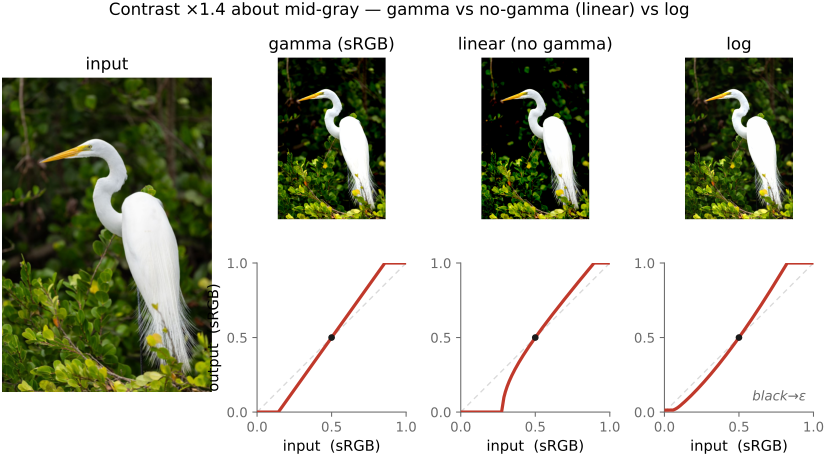
fig-point-op-contrast-spaces · the same contrast (×gain about mid-gray) in gamma (sRGB) / linear (no gamma) / log: three outputs + remapping curves (linear crushes shadows, log preserves them; black clamped to ε for log) 🟨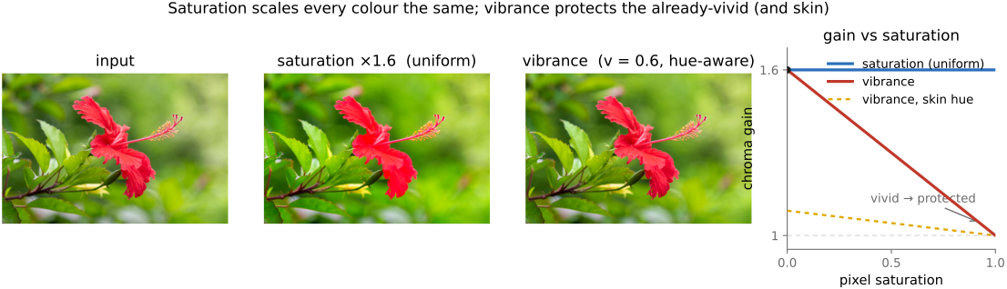
fig-point-op-saturation-vibrance · uniform saturation (constant `s`, over-saturates already-vivid colours → clip) vs vibrance (per-pixel gain `g = 1+v(1−sat)·w_skin(hue)`, protects vivid colours & skin): input, saturation, vibrance + a gain-vs-saturation panel (Point operations → Basic colour enhancement, BASIC) 🟩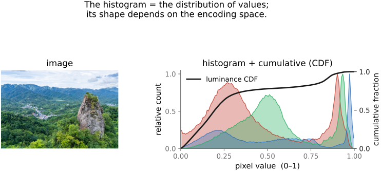
fig-histogram · an image histogram (per-channel) + cumulative histogram; its shape depends on the encoding space (BASIC tone mapping) 🟨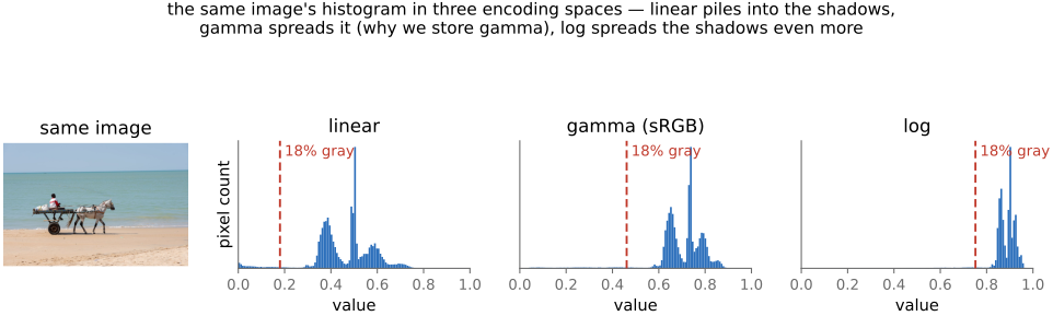
fig-histogram-encoding-spaces · the same image's luminance histogram in linear / gamma (sRGB) / log; 18% gray marked at 0.18 / ~0.46 / ~0.75 — the encoding reshapes the value axis (BASIC histograms) 🟩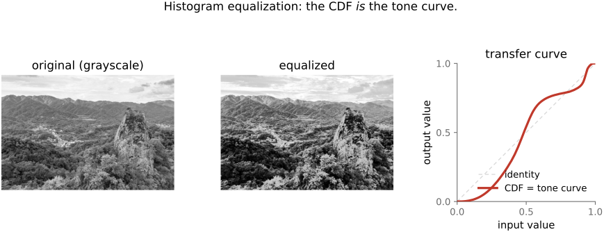
fig-histogram-equalization · histogram equalization — the CDF used as the transfer curve, before/after (BASIC) 🟨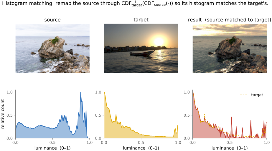
fig-histogram-matching · histogram matching — source + target images and their histograms → matched result, with the composed transfer curve $\text{CDF}_\text{tgt}^{-1}\circ\text{CDF}_\text{src}$ (BASIC histograms) ✅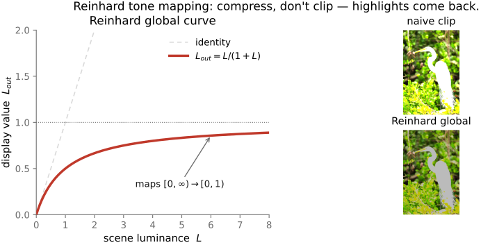
fig-reinhard-curve · the Reinhard global tone curve L/(1+L) mapping [0,∞)→[0,1); naive clip vs Reinhard on a simulated-HDR image (BASIC) 🟨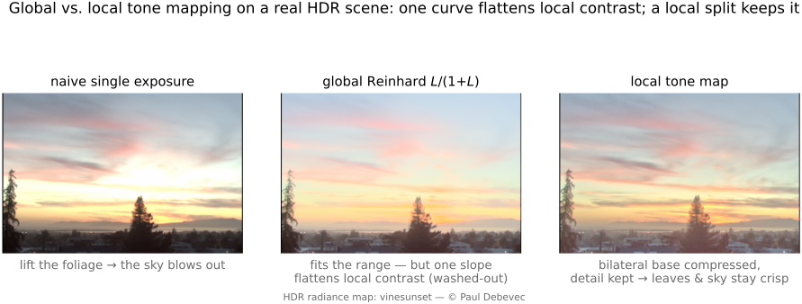
fig-tonemap-real · global vs local tone mapping RESULT on a real HDR photo (seal at marina): naive single exposure · global Reinhard (one slope flattens local contrast → hazy) · local bilateral base+detail split (range fits, detail stays crisp) — real-image companion to `fig-tonemap-global-vs-local` (BASIC tone mapping) ✅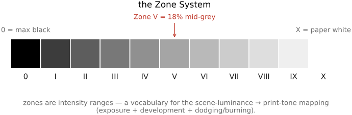
fig-zone-system · the Zone System strip 0–X, Zone V = 18% mid-grey (scene → print) (BASIC) 🟨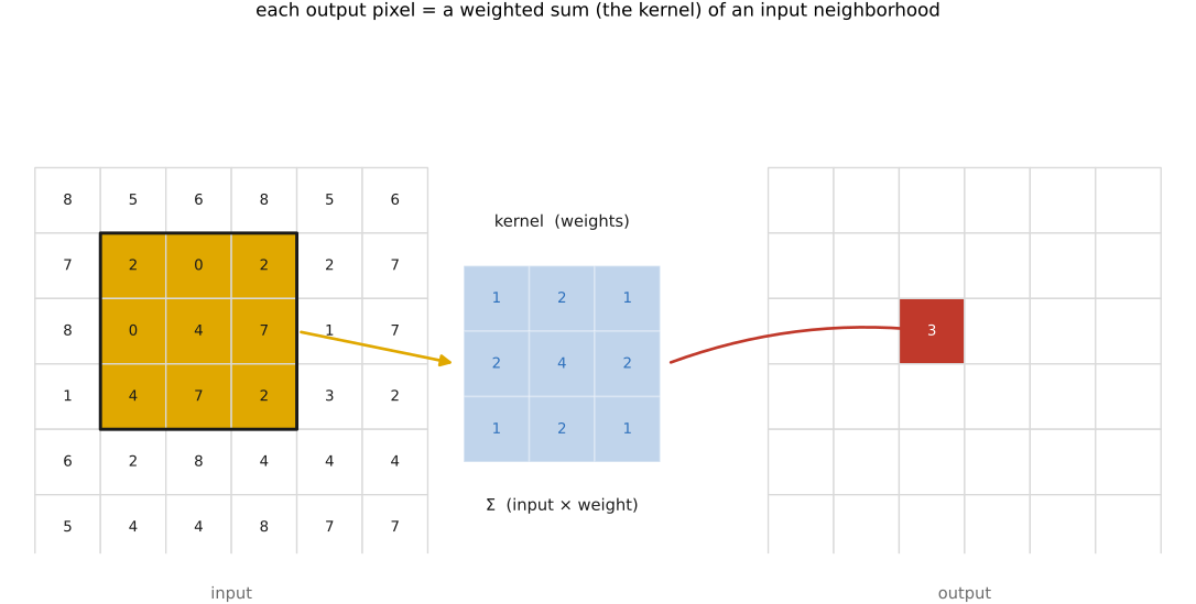
fig-convolution-slide · a kernel sliding over an image, weighted-summing a neighborhood into one output pixel (Convolution, BASIC) 🟨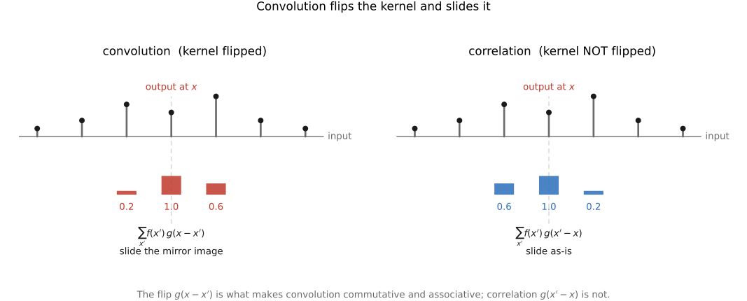
fig-convolution-flip · the flip: where-from vs where-to — convolution `g(x−x')` vs correlation 🟨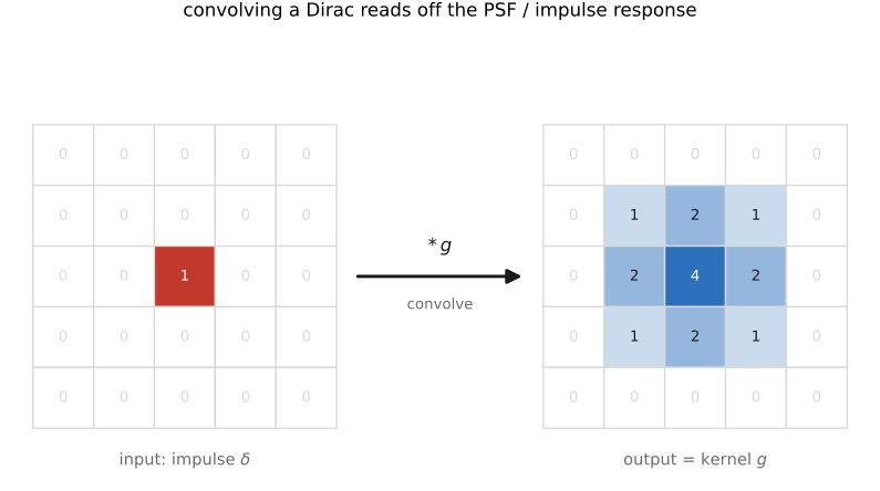
fig-psf-impulse · impulse in → kernel out: convolving a Dirac reads off the PSF / impulse response 🟨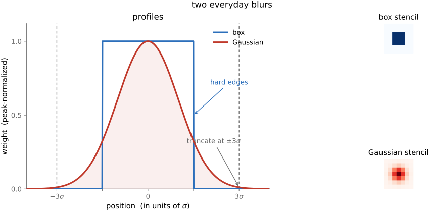
fig-blur-zoo · box vs Gaussian kernels — profiles + 2-D stencils, Gaussian truncated at ~3σ 🟨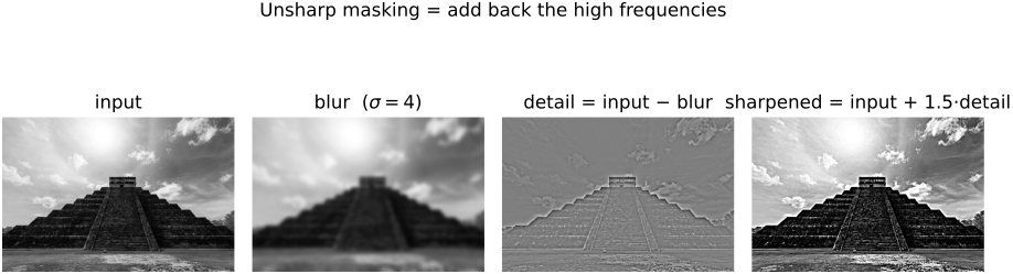
fig-unsharp-mask · unsharp-mask decomposition: input − blur = detail (high-pass), output = input + k·detail 🟨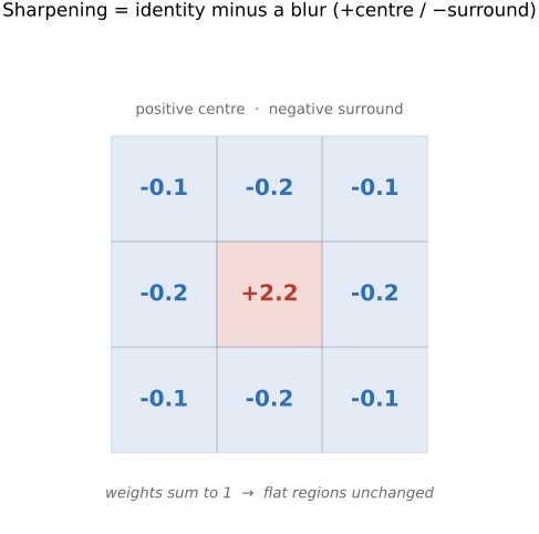
fig-sharpen-kernel · the sharpening kernel δ − blur as a +centre / −surround stencil 🟨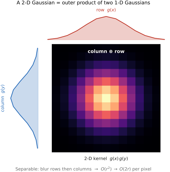
fig-separable · separability — a 2-D Gaussian = 1-D ⊗ 1-D (blur rows then columns); O(r²) → O(2r) 🟨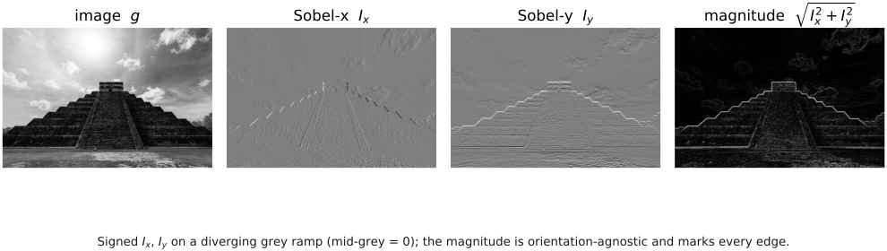
fig-gradient-sobel · Sobel x / y → gradient magnitude (edge strength) on an image 🟨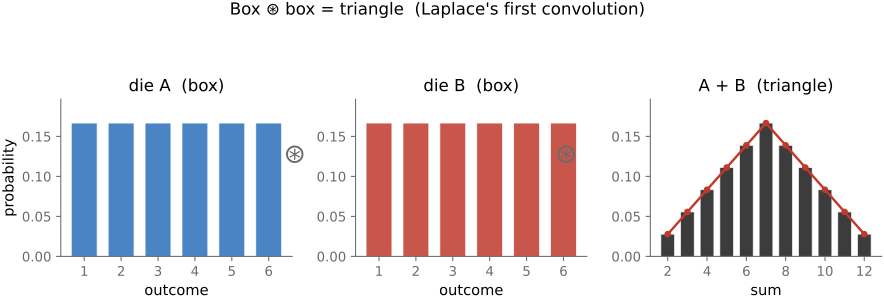
fig-convolution-probability · convolution as the sum of random variables: box ⊛ box = triangle (two dice) 🟨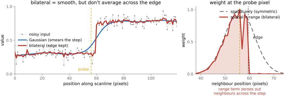
fig-bilateral-1d · noisy step edge: noisy input vs Gaussian (smears step) vs bilateral (denoises plateaus, keeps step); side panel — per-pixel spatial×range weight collapses to one side at the edge (Bilateral filtering) ✅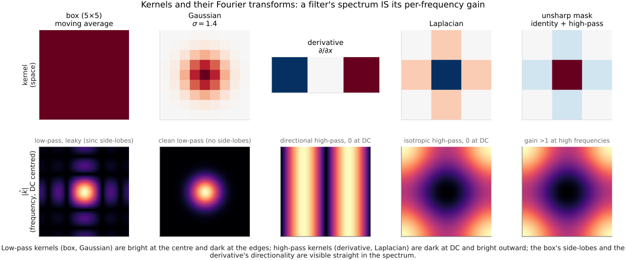
fig-kernel-spectra · five common kernels (box, Gaussian, derivative ∂/∂x, Laplacian, unsharp mask) shown in space and as their Fourier magnitudes — a filter's spectrum IS its per-frequency gain (low-pass leaky vs clean, directional/isotropic high-pass, boosting) ✅fig-unsharp-mask · unsharp-mask decomposition: input − blur = detail (high-pass), output = input + k·detail 🟨fig-sharpen-kernel · the sharpening kernel δ − blur as a +centre / −surround stencil 🟨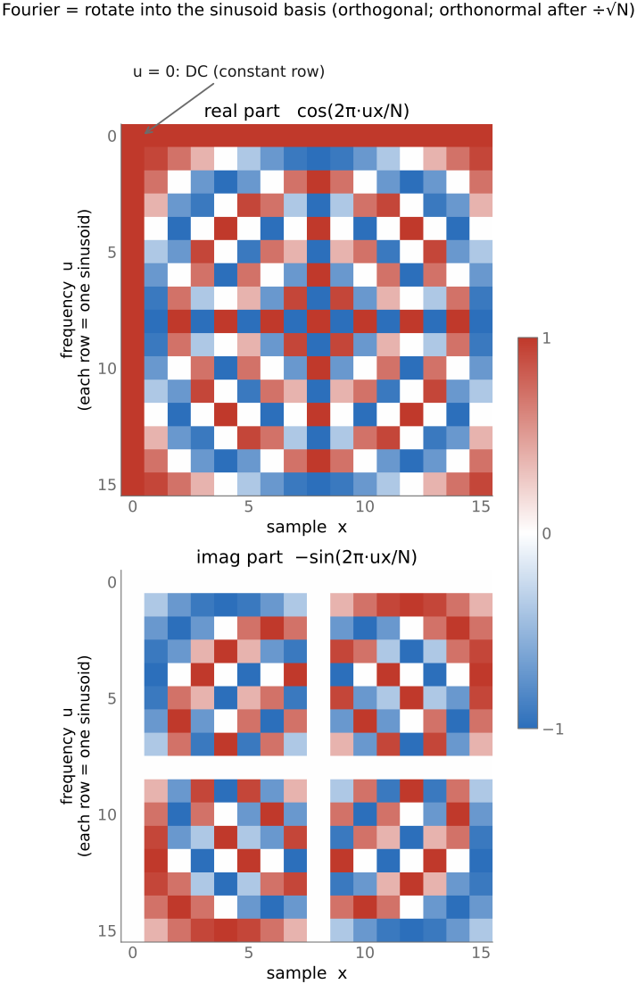
fig-fourier-basis-matrix · the DFT as a change-of-basis matrix (real & imaginary parts) 🟨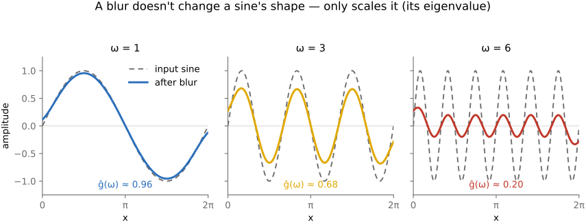
fig-sine-eigenvectors · sine waves are the eigenvectors of convolution: same wave out, only amplitude/phase change 🟨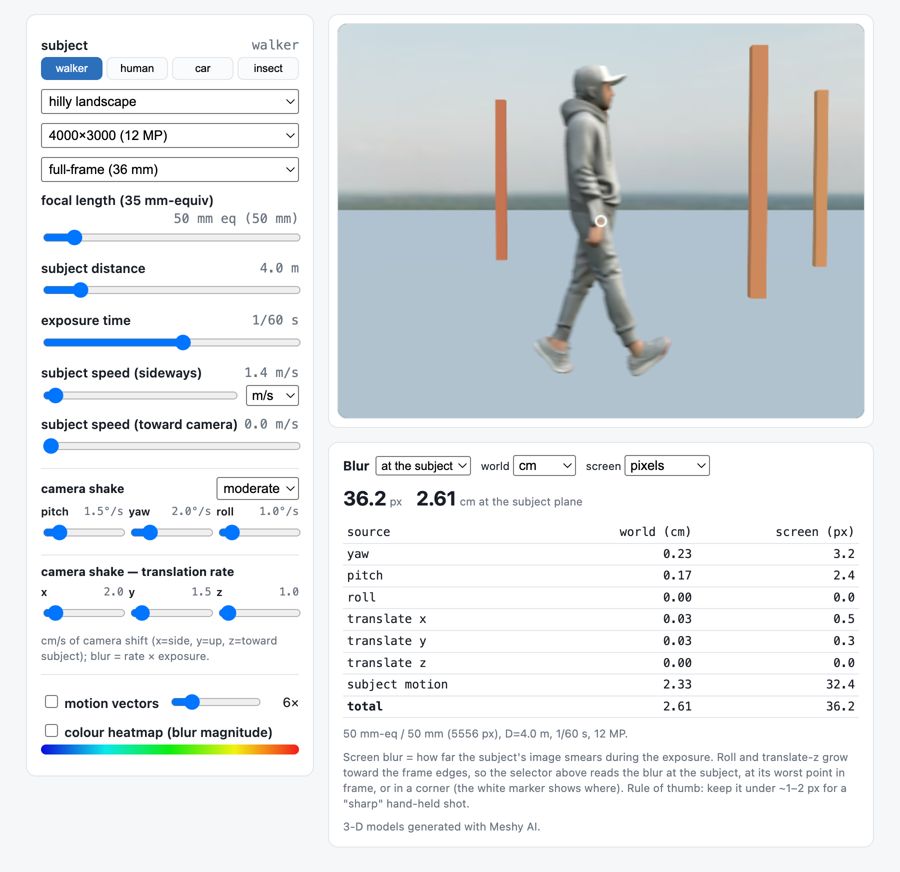
fig-motion-blur-calculator · live motion-blur calculator: a 3-D scene (walking figure or a car) imaged by a virtual camera, the blur rendered by **temporal supersampling** (many instants across the exposure, averaged). Set resolution / sensor / focal length (35 mm-equiv) / distance / exposure, add camera-shake **rates** in rotation (pitch/yaw/roll) and translation (x/y/z) plus a subject speed; the readout gives the blur at the subject in world (cm/m/in) and screen (px / % width) units, broken down by source. A per-pixel **G-buffer** (depth + subject mask) drives exact motion-vector arrows and a blur-magnitude heatmap: the subject carries its own motion, the background only camera shake. Environment backdrops + car colour picker. Static fallback is a screenshot. *3D models generated with Meshy AI.* ✅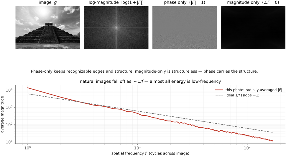
fig-fourier-magnitude-phase · an image's Fourier magnitude & phase, and the phase-swap demo (phase carries structure) 🟨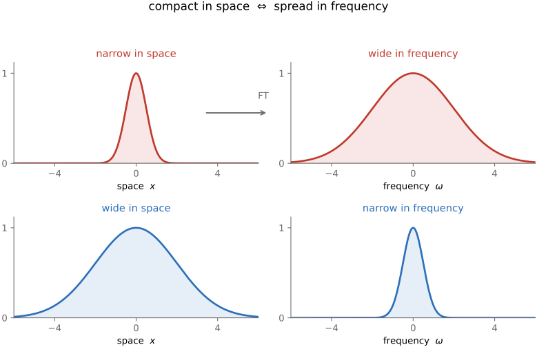
fig-compact-space-frequency · compact in space ⇔ spread in frequency (narrow vs wide Gaussian and its transform) 🟨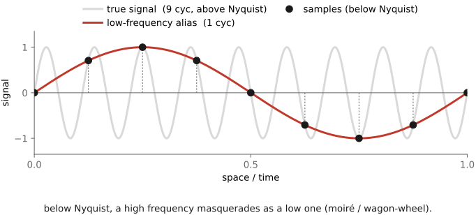
fig-aliasing · sampling a sine too coarsely → aliasing (high frequency folds to a low one) 🟨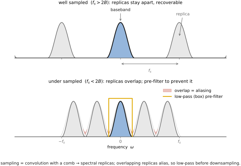
fig-sampling-comb · sampling = multiply by a comb → spectral replicas; pre-filter (low-pass) before downsampling 🟨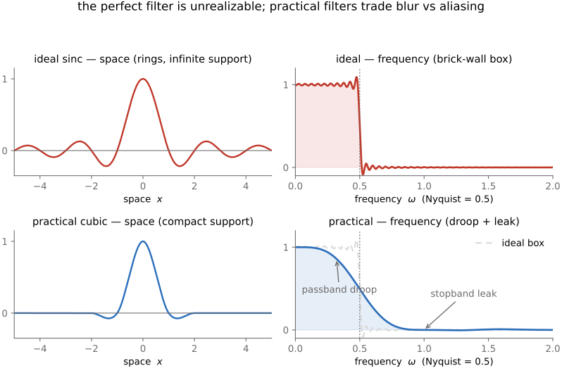
fig-sinc-vs-practical · ideal sinc reconstruction vs a practical filter, in space and frequency 🟨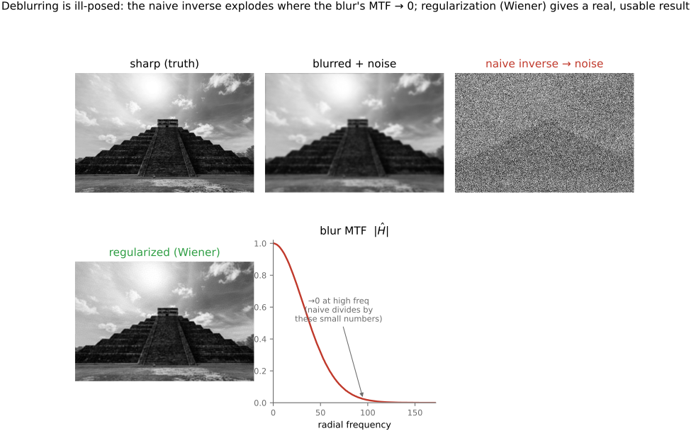
fig-deblur-preview · the deblur preview: sharp → blurred + noise → naive inverse amplifies noise; MTF 🟨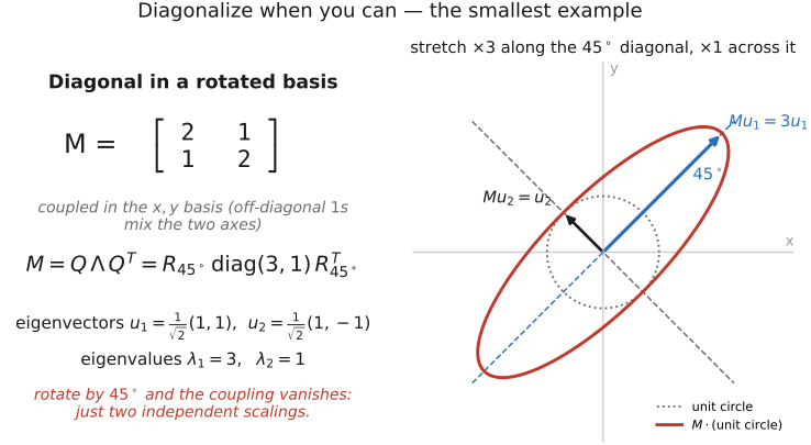
fig-diagonalize-2x2 · 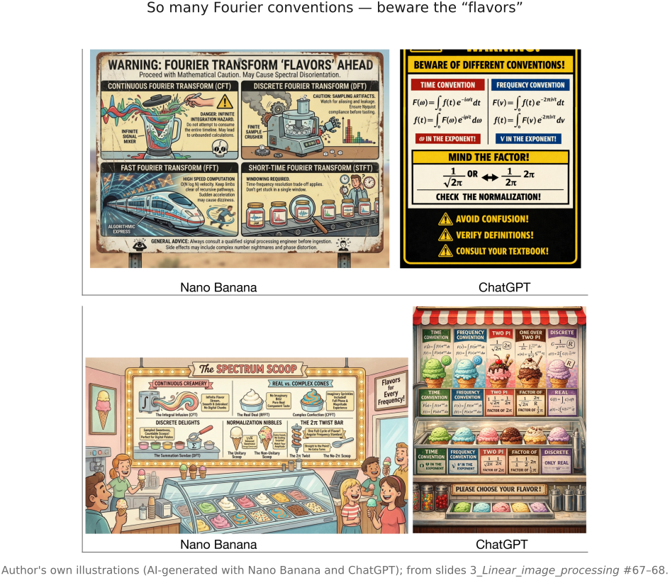
fig-fourier-conventions · 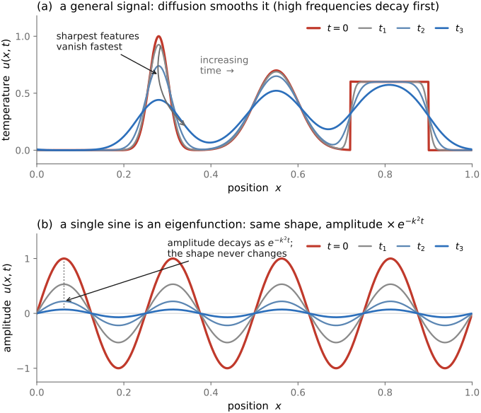
fig-heat-diffusion-1d · 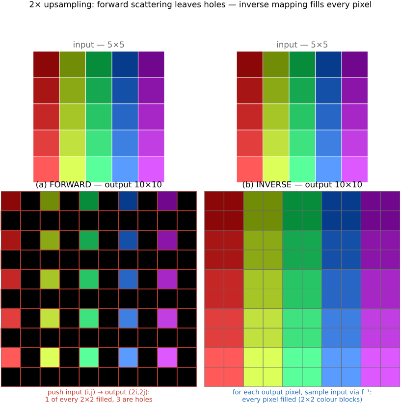
fig-resample-forward-inverse · concrete 2× upsampling on a 5×5 → 10×10 rainbow grid: FORWARD pushes input (i,j)→output (2i,2j) so 1 of every 2×2 output block is filled and 3 are black holes (regular lattice of gaps); INVERSE loops output, samples input via f⁻¹ (nearest) → every pixel filled (2×2 colour blocks). Forward leaves holes, inverse fills everything (Resampling, BASIC) ✅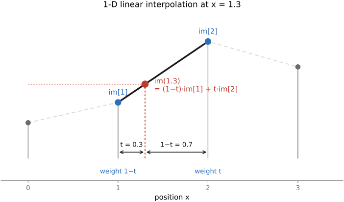
fig-linear-interp-1d · 1-D linear interpolation — `im[1.3]` from its two neighbours 🟨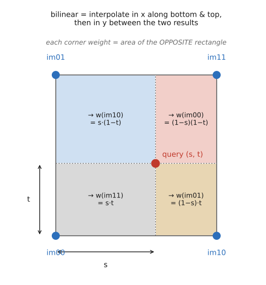
fig-bilinear · bilinear interpolation — the 4-neighbour weighting on the unit square 🟨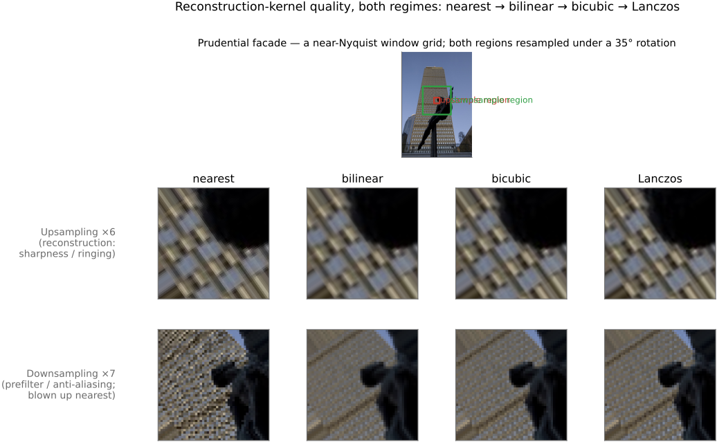
fig-resample-kernels-real · the kernel ladder on a REAL photo (Boston skyline + rainbow) resampled under a 35° rotation, magnified on a detail: nearest (blocky) → bilinear (smeared) → bicubic (edges restored) → Lanczos (sharpest) — adds Lanczos + the rotation case to `fig-interp-comparison` ✅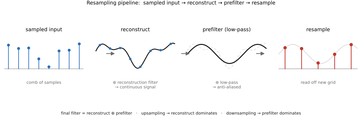
fig-reconstruction-pipeline · the resampling pipeline: sample → reconstruct → prefilter → resample 🟨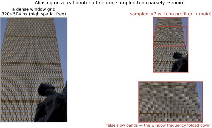
fig-aliasing-photo · aliasing/moiré on a real photo: a window-grid facade decimated with no prefilter folds into moiré bands — the 2-D, real-image companion to `fig-aliasing` (Sampling and aliasing) ✅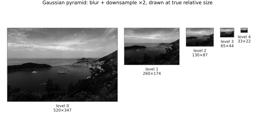
fig-gaussian-pyramid · the Gaussian pyramid — repeated blur + downsample tower (Pyramids, BASIC) 🟨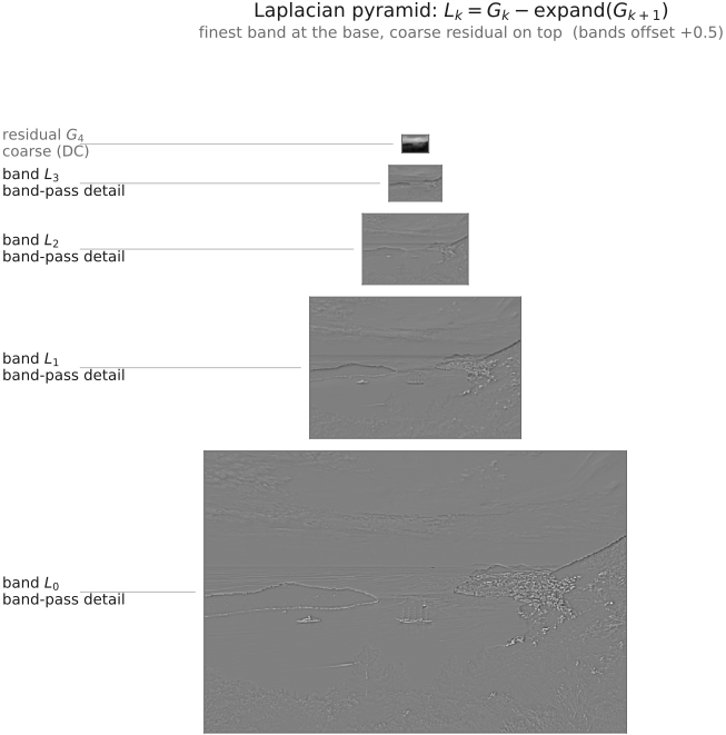
fig-laplacian-pyramid · the Laplacian pyramid — band-pass levels (G_k − expand(G_{k+1})) 🟨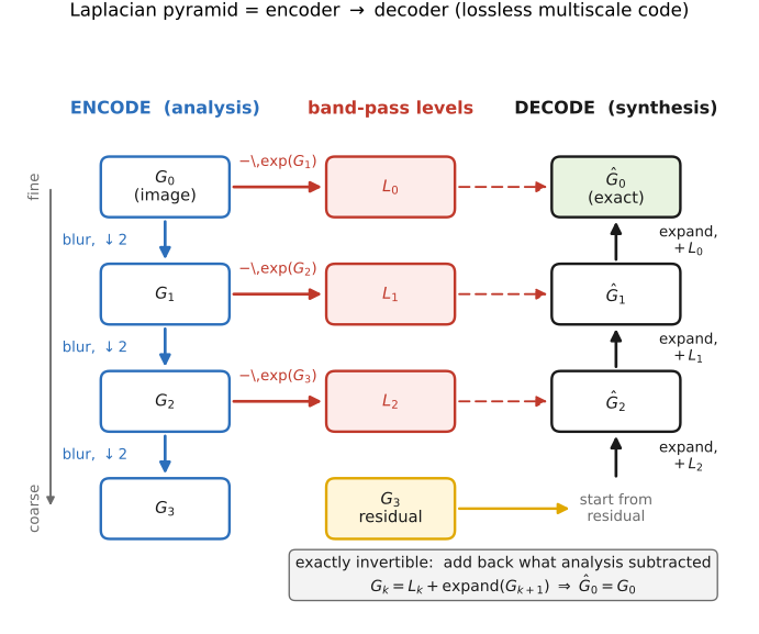
fig-pyramid-encode-decode · the Laplacian pyramid as an encoder → decoder (exact reconstruction) 🟨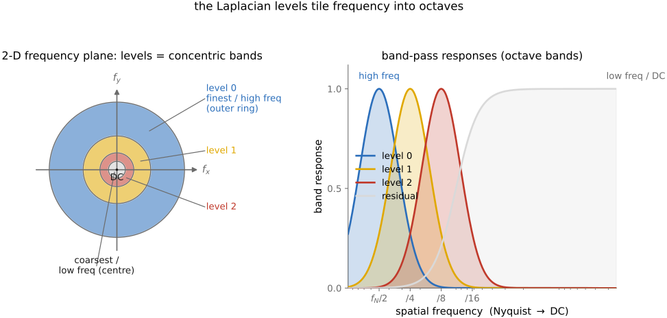
fig-pyramid-frequency-bands · each pyramid level = a frequency band (concentric Fourier rings) 🟨fig-kernel-spectra · five common kernels (box, Gaussian, derivative ∂/∂x, Laplacian, unsharp mask) shown in space and as their Fourier magnitudes — a filter's spectrum IS its per-frequency gain (low-pass leaky vs clean, directional/isotropic high-pass, boosting) ✅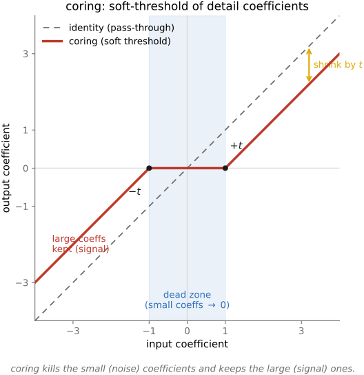
fig-coring · coring — zero the small detail coefficients (noise), keep the large ones 🟨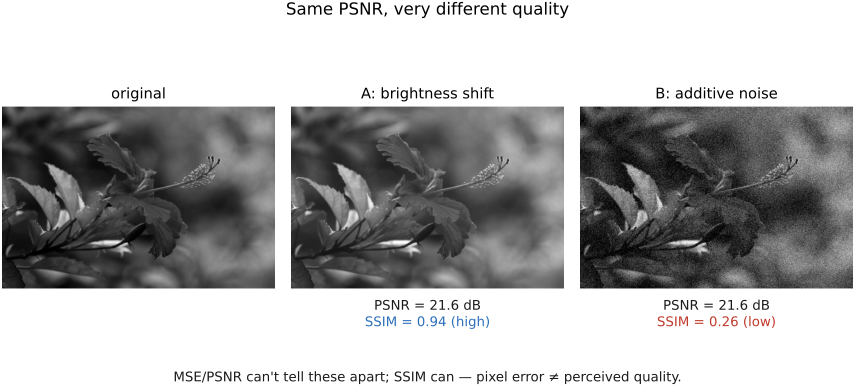
fig-ssim-vs-mse · same PSNR, very different SSIM — pixel error ≠ perceived quality (Image metrics, BASIC) 🟨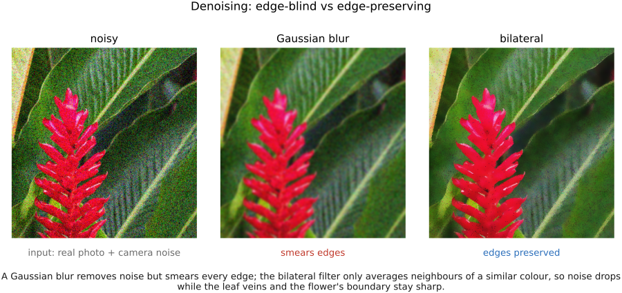
fig-denoising-before-after · denoising a real colour crop (realistic shot+read noise): noisy vs Gaussian (smears edges) vs bilateral (edge-preserving) (Denoising, BASIC) ✅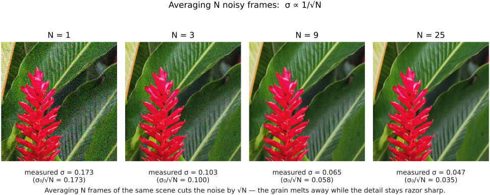
fig-averaging-convergence · averaging N noisy frames → noise drops as 1/√N (1, 3, 9, 25 frames), on a real colour photo with realistic shot+read noise (Denoising, BASIC) ✅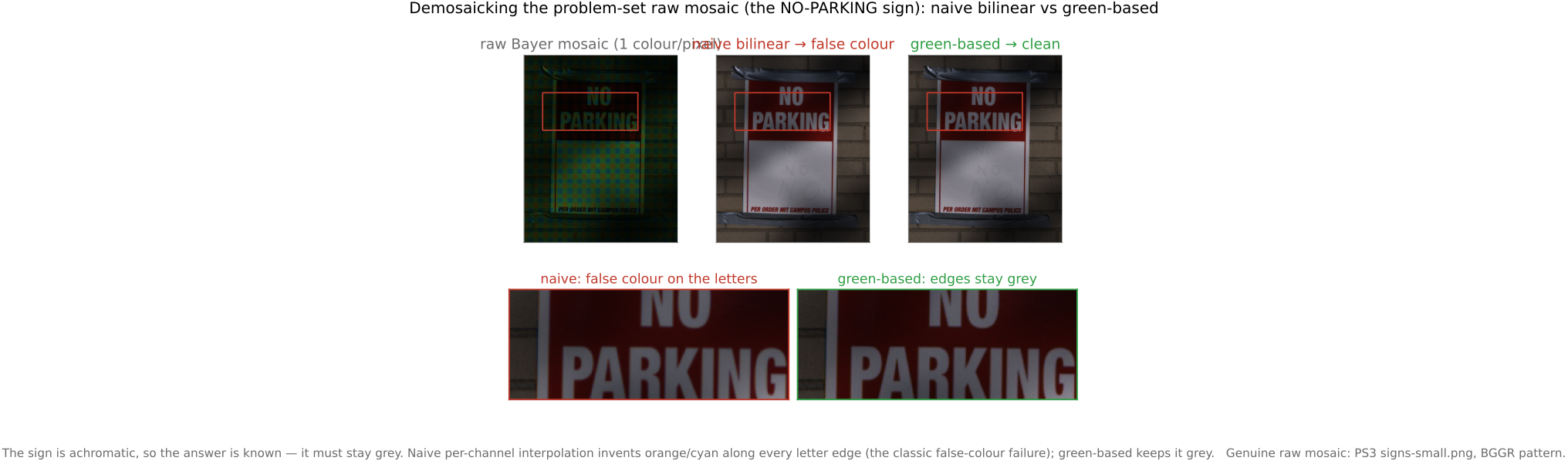
fig-demosaick-real-bayer · the PS3 raw mosaic (NO-PARKING sign) demosaicked: ground truth · simulated RGGB Bayer mosaic · naive bilinear (false colour on the window grid) · green-based (clean), with a zoom (Demosaicking, BASIC) ✅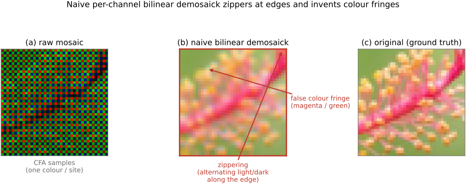
fig-demosaick-before-after · Bayer → RGB: the mosaic, naive bilinear demosaick (zipper / fringing), edge-aware (Demosaicking, BASIC) 🟨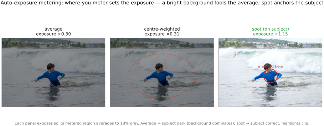
fig-ae-metering · **interactive** AE metering modes: pick a scene + mode (average / centre-weighted / movable+resizable spot); the demo exposes so the metered region averages 18% and reports metered tone, gain, and clipped %; "where you meter sets the exposure" ✅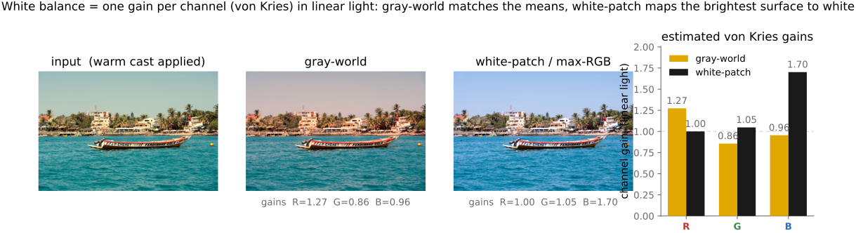
fig-white-balance-real · white balance computed from scratch (von Kries per-channel gain in linear light): a warm-casted photo corrected by gray-world vs white-patch/max-RGB, with the recovered channel gains (PS1) ✅fig-wb-before-after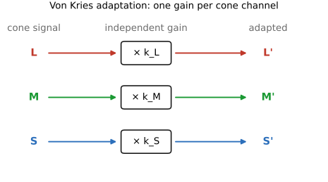
fig-von-kries · Von Kries per-channel gains 🟨fig-illuminant-metamerism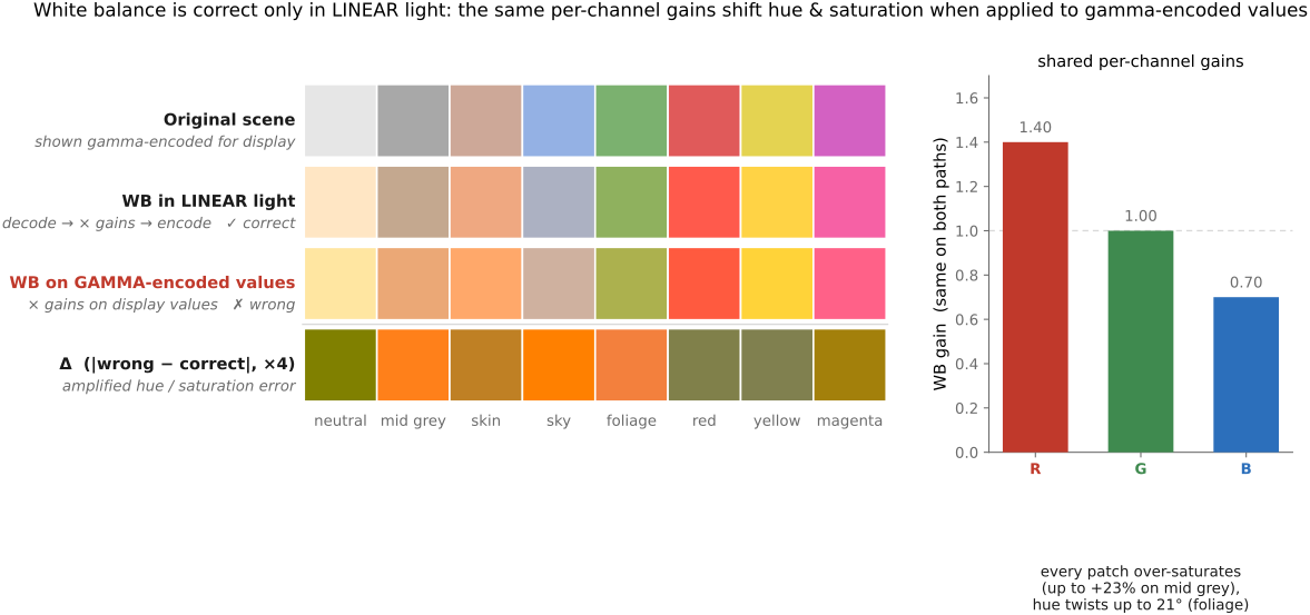
fig-wb-linear-vs-nonlinear · 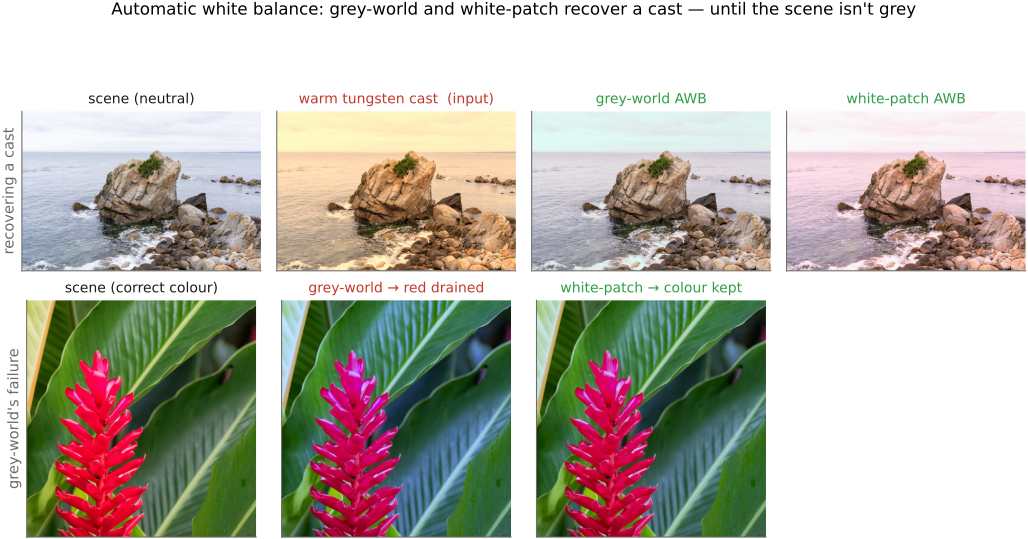
fig-awb-greyworld · AWB as results: grey-world & white-patch recover a warm tungsten cast on a neutral scene; grey-world drains the colour on a colour-dominant scene while white-patch survives (the assumption is the algorithm) ✅fig-awb-mixed-fail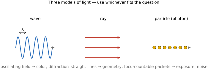
fig-light-models · three models of light: wave (λ) vs ray vs particle/photon propagation, and what each is good for 🟨fig-mixed-illuminant-scene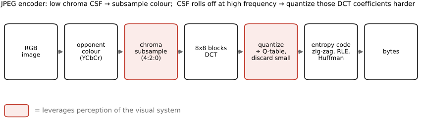
fig-jpeg-pipeline · the JPEG encoder — RGB → opponent colour → chroma subsample → 8×8 DCT → quantize → entropy code (File formats, BASIC) 🟨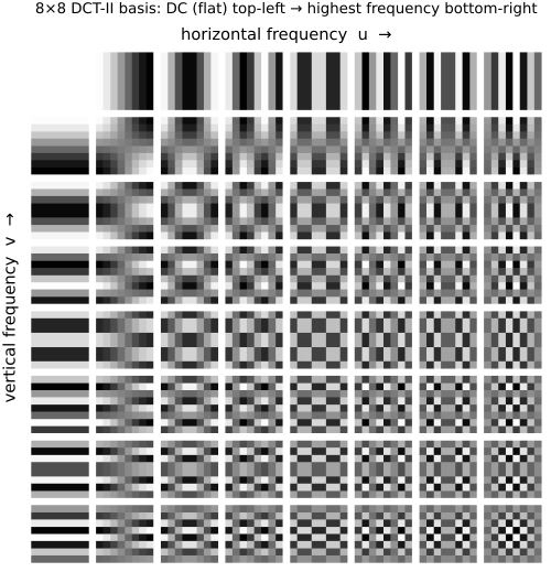
fig-dct-basis · the 8×8 DCT-II cosine basis (DC top-left → high frequency bottom-right) 🟨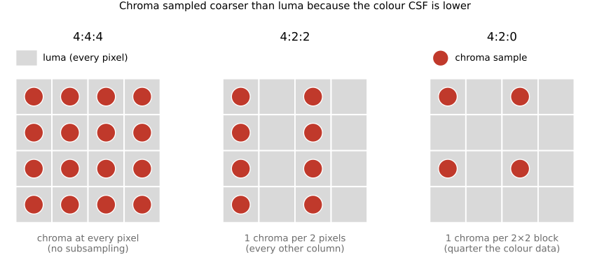
fig-chroma-subsampling · chroma subsampling grids 4:4:4 / 4:2:2 / 4:2:0 (chroma sampled coarser than luma) 🟨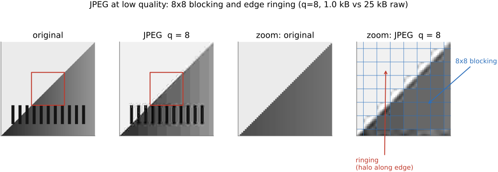
fig-jpeg-artifacts · JPEG blocking & ringing at low quality (original vs q=8, zoomed crop) 🟨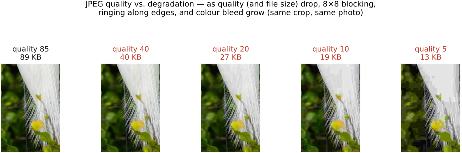
fig-jpeg-quality-levels · JPEG quality sweep (q=85→40→20→10→5): the same photo's edge-crop at each quality with the whole-image file size beneath — degradation grows as size drops (File formats, BASIC) 🟩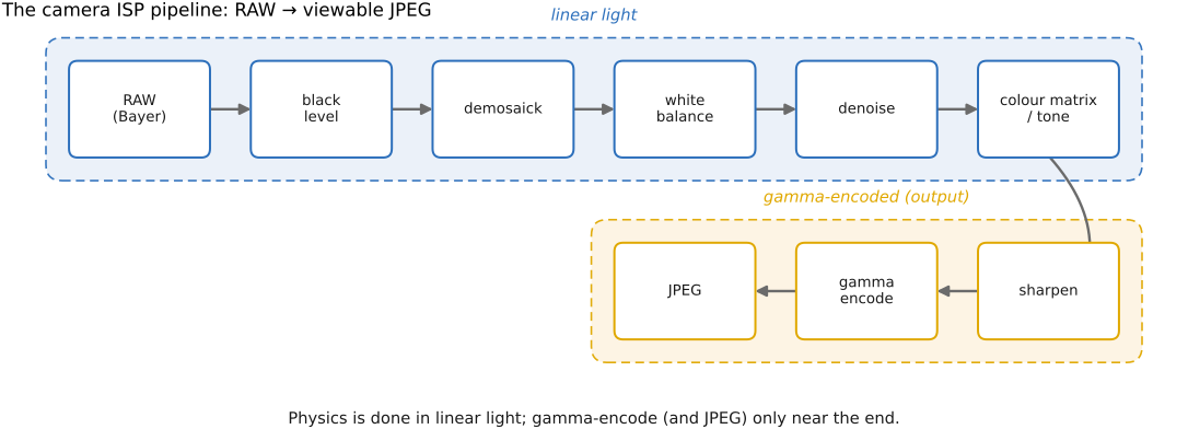
fig-isp-block-diagram · the ISP pipeline: RAW → black level → demosaick → white balance → denoise → tone/colour → sharpen → gamma → JPEG (Recap ISP, BASIC) 🟨