draft · v0.1.226
💬Comments welcome. To leave a note, select any text and click the note / highlight button that pops up — or open the panel with the tab at the top-right (‹). Notes are visible only inside our private review group.
Computational Photography, an AI-powered Slopendium
Frédo Durand, MIT · Version 0.2.52
expand to30 parts · 288 chapters · 1329 sections · 665 figures embedded · 142 placeholders · double-click a figure to enlarge
Part 1 INTRO
1.1 From Digital to Computational Photography
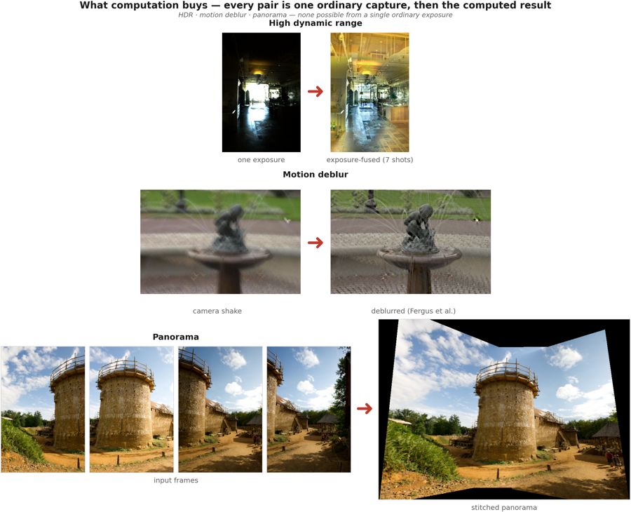
fig-results-montage
fig-results-montage · a montage of computational-photography results — HDR tone mapping, refocus-after-capture, motion deblur, a stitched panorama — the "look what computation buys you" opener
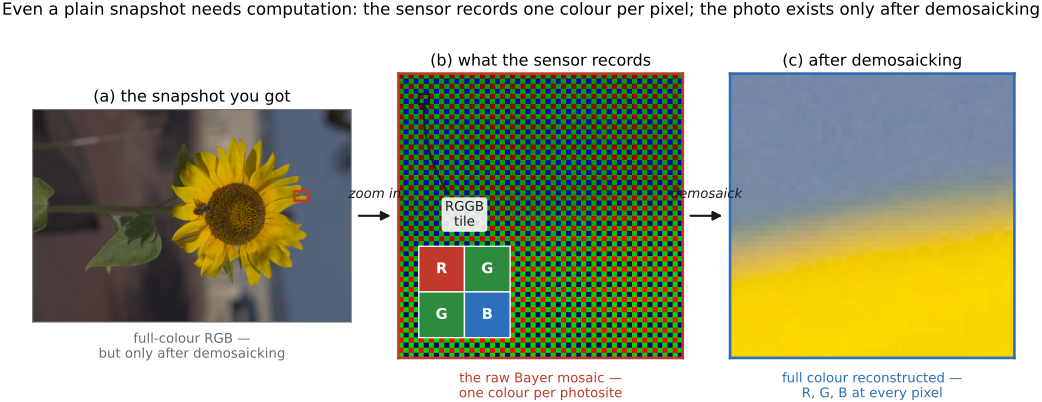
fig-demosaick-snapshot
fig-demosaick-snapshot · even a plain snapshot needs computation: one colour per pixel (Bayer mosaic) → demosaicked RGB
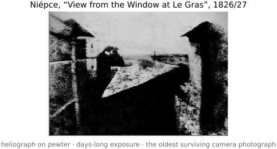
fig-first-photograph
fig-first-photograph ·
At first, the digital revolution merely replaced film by digital sensors more amenable to quick snapshots, instant gratification and sharing. But it did more than that : it created the opportunity to add arbitrary computation between the photons in a scene and the final image.
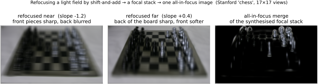
This allows us to do really cool stuff : manage scenes where contrast is excessive, computationally remove blur, combine images into virtual wide angle panoramas, and even capture the full array of light to do stuff like refocusing after the fact and extract 3D.
[results-montage figure — HDR tone mapping (Durand et al.), refocus-after-capture (Ng et al.), motion deblur (Levin et al.), panorama (problem set)]
In fact, even a simple snapshot requires serious computation because each pixel usually captures only one of the 3 channels and the other two need to be reconstructed [demosaick-snapshot figure]. Cell phones these days take much better images than they have a right to because of computational photography.
Plus generative AI is poised to further revolutionize photography and image making with its ability to learn the space of all possible images in a manner reminiscent of a Borges novella (cite *The Library of Babel* and https://arxiv.org/abs/2310.01425)
1.1.3 What makes a technique useful
1.1.5 Does photography still matter in the age of generative AI?
1.1.8 Neighbouring fields, and where the work is published
1.2 How to read this book
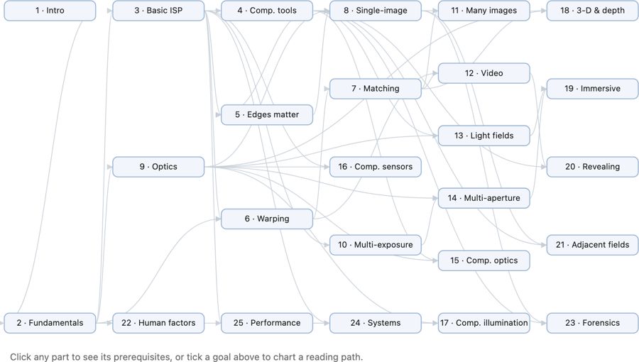
fig-chapter-dependency-graph
fig-chapter-dependency-graph · graph of chapter dependencies (provides/requires) so a reader can chart a path 🟨
• the book is organized **cross-cuttingly**: a chapter is sometimes a **tool** (convolution, the bilateral filter), sometimes a **big idea** (priors, the light field), and the major themes deliberately **recur** across chapters — the same lesson seen from several angles. The redundancy is intentional; cross-references thread the pieces together.
• **hammers and nails**: we deliberately sought a **balance between "hammers and nails"** — between **tools/techniques** (the hammers: convolution, the bilateral filter, optimization, priors) and **applications/challenges** (the nails: HDR, panoramas, deblurring, refocusing). Rather than a purely tool-first or purely application-first table of contents, the book's structure is **organized by a combination of tools and applications/challenges**, alternating between the two so each motivates the other.
• **intuition first**: lead with the idea and a picture, then the math. The audience is a **CS undergrad**, new to imaging (what to know coming in is spelled out in *[[#Prerequisites]]* below).
• **how to read**: FUNDAMENTALS grounds the physics and perception; BASIC IMAGE PROCESSING gives the toolkit; later parts build single- and multi-image computational photography. Read mostly front-to-back, or follow the dependency graph below to chart your own path.
• **how this book came to be**:
• grew out of Frédo's **computational photography course** at MIT — its lectures, slides, and problem sets are this book's backbone.
• written **with an AI collaborator** (Claude) as a deliberate experiment in **AI-assisted authoring** — the outline, figures, drafts, and the book's own tooling were co-developed; a fitting, slightly meta nod to the generative-AI theme the book itself discusses.
• the **process** (how outline, figures, and prose are generated, verified, and kept consistent) is documented in an appendix — itself a small piece of AI methodology [forward ref: "how this book was created"].
• **chapter dependency graph**:
• *(placeholder — to create later)* a **graph of chapter dependencies** belongs here, at the end of the intro: a diagram showing which chapters rely on which, so a reader can chart their own path through the book. Generate it from the **provides / requires** graph (see [[Book Generation Process#Cross-chapter dependencies]] and each section's `- prereqs:`), once enough of the book is written for the dependencies to be stable.
1.2.1 A book for machines, too
1.3 How this book was made
• a **short, intro-level** chapter (the headline version of the appendix [[Appendices#How this book was created]]): the book is partly *about* generative AI and was partly written *with* it, so the making-of is part of the story, not a footnote.
• **where it came from**: grew out of Frédo's MIT computational photography course — ~**305k words** of auto-captured/auto-transcribed lecture transcripts, ~**114k** of slide decks, ~**42k** of problem sets (~**460k** of pre-existing teaching material) form the backbone.
• **how it was written**: drafted **with an AI collaborator** (Claude); outline/prose split with a compile step; figures are programs; the human edits triage back so re-compiling reproduces the corrections.
• **who did what**: AI for laborious-but-specified drafting, figure code, and bookkeeping; human for structure, judgment, catching subtle errors, and ownership of every claim.
• **the numbers, honestly**: ~**40.5k words** of typed prompts steered ~**735k words** of generated outline+prose (≈13–18× leverage, *not* authorship); the outline is model output too, so the earlier "2.2× human writing" framing was wrong — the real human contribution is **curation**, not keystrokes. Point to the two appendices for the full account and the under-the-hood prompts/verifiers.
1.4 What programming language for computational photography?
• the book is **language-agnostic in its ideas** but ships in two editions — a **Python** one and a **C++** one (never one book showing both) — because the two languages serve different moments: Python to *think and prototype*, C++ to *ship and run fast*. The concepts are identical; pick the edition that matches your goal.
• **why choose which**: **Python** for **deep learning, prototyping, and convenience**; **C++** for **performance**. The gap is not small. When you write the **low-level code yourself** (e.g. your own convolution rather than a library call), the **speed differential** is dramatic: in Frédo's experience, roughly **1000× from Python to optimized C++**, and **at least another ~10× from C++ to Halide**. So the language choice is also a performance choice — see [[Performance engineering and Halide]] and [[Appendices#Programming: Python, C++, and PyTorch]].
• **Python** — the right default for *learning, prototyping, and research*:
• **pros**: **readable** — NumPy array code reads almost like the math (`out = a + 0.5*b`); **fast to write and explore**, with interactive notebooks and instant feedback; a vast **ecosystem** (NumPy, SciPy, Pillow / OpenCV, scikit-image, Matplotlib, and the whole deep-learning stack — PyTorch, JAX); automatic memory; the lingua franca of research and ML.
• **cons**: **slow at the pixel level** — a naive per-pixel Python loop is orders of magnitude slower than C, so you must **vectorize** (push the loop down into NumPy's C core) or it crawls; the **GIL** limits real CPU threading; packaging / deployment is awkward; dynamic typing lets type bugs hide until run time; little control over memory layout or exact performance.
• bottom line: the right default for **learning, prototyping, and research** — and, through NumPy / PyTorch, fast *enough* for most of what we do here.
• **C++** — the right default for *performance and production*:
• **pros**: **fast and predictable** — close to the metal, with control over memory layout, cache behaviour, and SIMD; what real **camera ISPs, real-time pipelines, and shipped products** are written in; static types catch errors at compile time; deploys to phones and embedded hardware.
• **cons**: **verbose and slower to write**; **manual memory management**, a rich source of bugs (out-of-bounds, leaks, use-after-free); a heavier **build / toolchain** story; far less interactive (edit–compile–run, not edit–run). The productivity tax is real.
• bottom line: the right default for **performance and production** — once the algorithm is settled and it must run fast, on device, at scale.
• **Halide** — a **domain-specific language** (embedded in C++ / Python) for high-performance image processing: you write the **algorithm** (what each pixel computes) **separately** from the **schedule** (how to tile, vectorize, parallelize, and fuse it across the memory hierarchy).
• **pros**: near-hand-tuned speed **without** hand-writing the tangled, hardware-specific loops; the *same* algorithm retargets to CPU / GPU / DSP by swapping the schedule; the basis of real camera stacks.
• **cons**: another language and mental model to learn, best reserved for the **hot paths** you have already identified — premature scheduling is its own trap. Covered properly in [[Performance engineering and Halide]].
• **MATLAB (historical note)**: for years *the* platform for this work — a strong numerical/linear-algebra library and an IDE that handled **images natively** (an image is a matrix; `imread`/`imshow`/slicing; the Image Processing Toolbox); much of the literature was prototyped in it. **Largely displaced by Python** (NumPy fills the same array niche, free) and especially **PyTorch** (autodiff + GPU + deep learning, which MATLAB never matched). Worth knowing because older papers/code are in it, and its array-thinking carries over to NumPy.
• **Libraries (implement-from-scratch, then build on)**: the book has you **implement core algorithms from scratch** to understand them (the `imageops` reference), but to *build* / dive into advanced projects, stand on mature libraries — **Python**: Pillow (PIL), NumPy/SciPy, OpenCV, scikit-image, PyTorch (also a GPU-array + autodiff engine); **C++**: OpenCV (de-facto standard), Eigen (linear algebra), LibRaw (raw decode), Halide (hot paths).
• **side bar — Photoshop 1.0, in 128,000 lines (a language lesson from 1990)**: Adobe (via the **Computer History Museum**, 2013) released the source of **Photoshop 1.0.1** — **≈128,000 lines across 179 files**, written for the Macintosh by **Thomas Knoll** (its sole engineer for v1 — a computer-vision PhD student whose 1987 image-display hack became the app). The language split *is* this section's lesson, 35 years early: **≈75 % Pascal** (the productive high-level language) and **≈15 % hand-written 68000 assembly** for the speed-critical inner loops — *most of it readable, the hot pixels hand-tuned* — exactly the Python-vs-C++/Halide trade-off (a high-level language for the bulk, machine code where it counts; what **Halide** now automates). The code is famously *mostly uncommented but well-structured*. It's now studied as a cultural artifact: the **"Das digitale Bild"** project (DFG / LMU Munich) runs an ongoing **Critical-Code-Studies** *"reading the source code of Photoshop"* — code as a text to be close-read. **For scale:** today's Photoshop is reportedly **millions** of lines of C++ (Frédo's estimate ~**10 M**); **Adobe Camera Raw (ACR)** and **Lightroom** share the same Camera Raw engine, and a typical camera **ISP** is a large proprietary C/C++ codebase — exact modern sizes mostly **not public** [⚠️ confirm the ~10 M / current ACR/Lightroom/ISP figures]. (→ the hand-tuned-inner-loop angle returns in [[Performance engineering and Halide]].)
• **Vibe coding (LLM-assisted)**:
• writing image code with an **LLM** ("vibe coding") is now part of the toolkit: great for **boilerplate, I/O, visualization, and explaining errors**, and a quick way to draft a function or a test.
• **but** image code is **numerically and perceptually subtle** — "looks plausible" is not "correct" — so keep the model on a **short leash** for filtering, resampling, color, and antialiasing, and always **verify against a hand-checkable input** (a constant, an impulse, a half-plane) before trusting it. Treat generated image code as *guilty until tested* (see [[Developing, Testing and Debugging]]). AI coding sometimes **fumbles the trivial** even when it nails the hard parts — see the cross-fade anecdote in [[Basic image processing and ISP#Vibe coding: writing image code with an LLM]].
1.4.1 On the desktop: Python, C++, and Halide
1.4.2 In the browser: JavaScript and the web stack
1.4.3 On the phone: Android and iOS
1.4.4 Libraries
1.4.5 Vibe coding
1.5 Problem sets
• **PS0 — Environment & C++ basics**: toolchain setup, a minimal `Image` class, image I/O. (→ [[Developing, Testing and Debugging]])
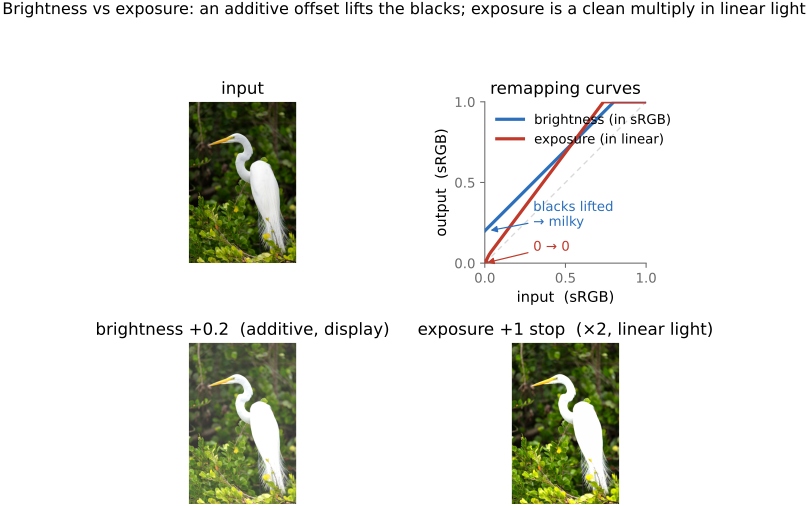
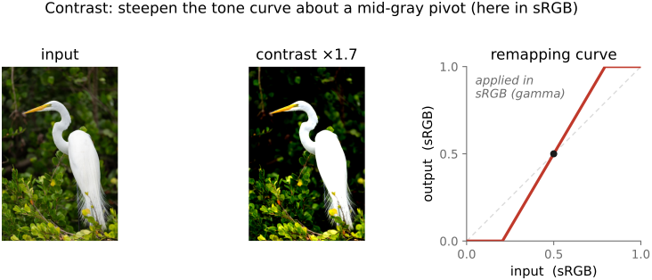
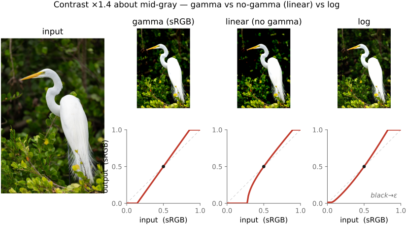
• **PS1 — Image class, point operations, color**: pixel access, brightness/contrast, luminance–chrominance (YUV), gamma, white balance, the Spanish-Castle illusion. (→ [[Image representation]], [[Point operations]], [[Perceptual color and trichromatic vision]])
• **PS2 — Convolution & the bilateral filter**: box/Gaussian blur, gradients, sharpening, and bilateral denoising (with a YUV variant). (→ [[Neighborhood operations and convolution]], [[Bilateral filtering]])
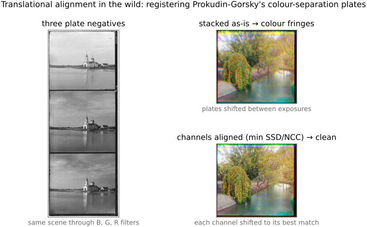
• **PS3 — Denoising & demosaicking**: align-and-average a burst, ISO/variance; Bayer demosaicking (green-first, edge-based, color-difference) and Prokudin-Gorsky channel alignment. (→ [[Denoising basics]], [[Demosaicking]])
• **PS4 — HDR**: merge an exposure bracket into a radiance map and tone-map it. (→ [[HDR merging]], [[Global tone mapping]])
• **PS5 — Resampling, warping & morphing**: nearest/bilinear/bicubic/Lanczos resampling; Beier–Neely segment warps; a full Beier–Neely morph. (→ [[Warping]], [[Morphing]])
• **PS6 — Homographies & manual panoramas**: homogeneous coordinates, warp by a homography, solve $H$ from four correspondences, stitch a planar mosaic. (→ [[Manual panorama stitching from multiple views]])
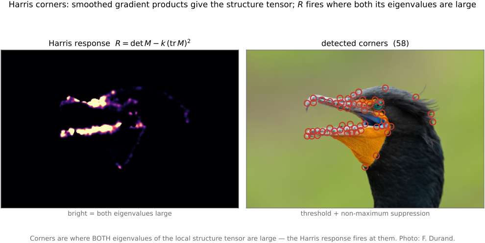
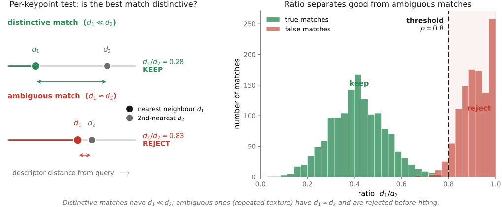
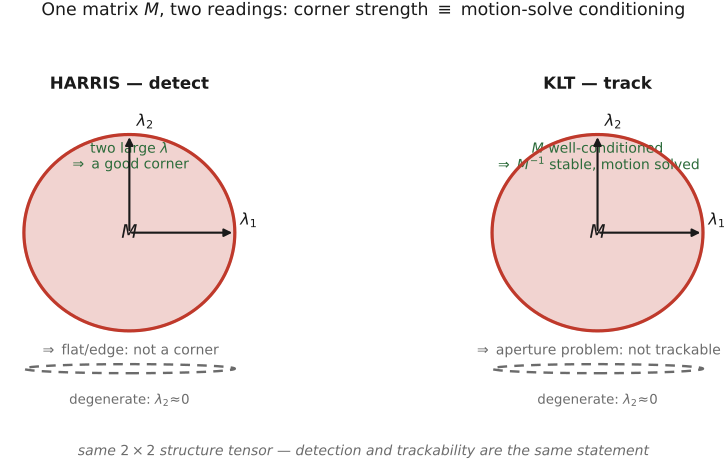
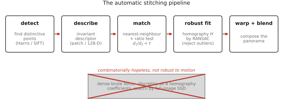
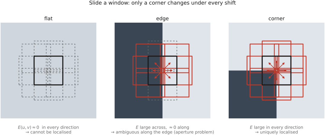
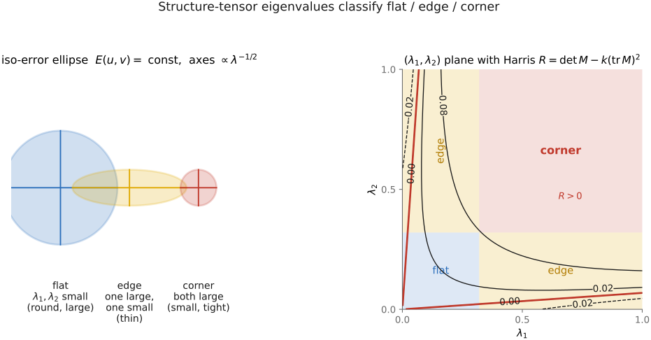
• **PS7 — Automatic panoramas**: Harris corners (structure tensor), patch descriptors, the second-nearest-neighbour ratio test, RANSAC, and feathered / two-scale blending. (→ [[Automatic panorama stitching from multiple views and feature matching]])
• **PS8 — Non-photorealistic rendering**: paintbrush splatting; single-scale, two-scale, and gradient-oriented painterly rendering. (→ [[Non-photorealistic rendering]])
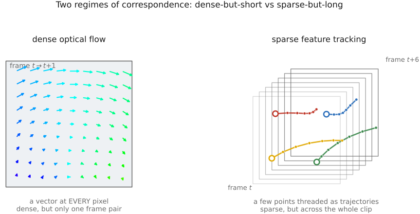
• **PS9 — Make-your-own / video & ethics**: a self-proposed project (optical-flow retiming, phase-based video magnification, …) plus the ethics deliverable; its open menu of advanced topics seeds many [[Computational optics and coded imaging]] sections. (→ [[Optical flow]], [[Motion and video magnification|Video magnification]])
Part 2 FUNDAMENTALS OF IMAGING
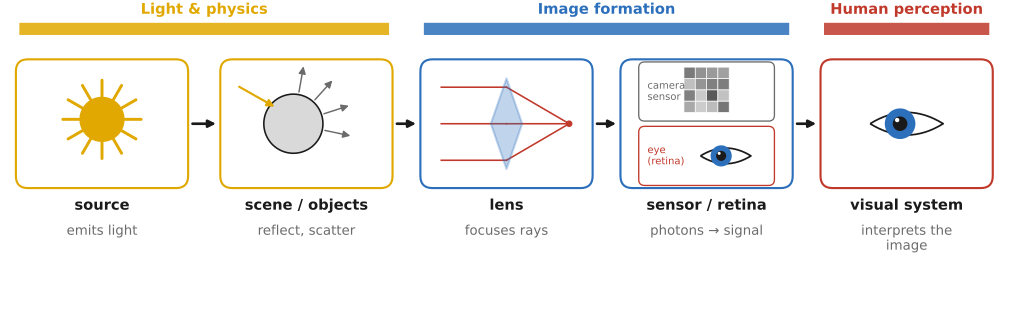
fig-light-journey
fig-light-journey · FUNDAMENTALS part opener — the journey of light: source → scene (reflection) → lens → sensor / retina → visual system, each step labelled with its chapter
**Photography means writing with light** — from the Greek *phōs* ("light") and *graphē* ("drawing"). This first part follows light on its entire journey and studies each step in turn.
• **the path of light** (and the chapters that follow it): a **source** emits light → it strikes **objects** and is reflected, absorbed, and scattered (the scene) → it passes through a **lens** → it lands on a camera **sensor** or the **retina**'s cones and rods → and the **visual system** interprets it.
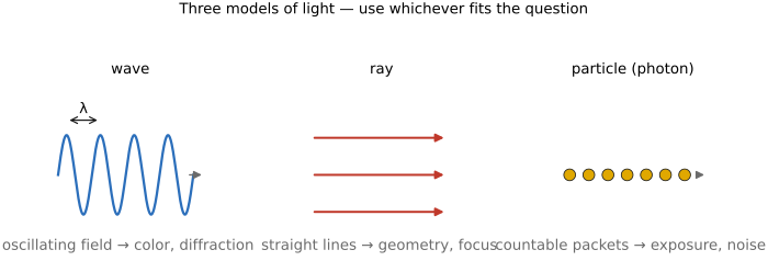
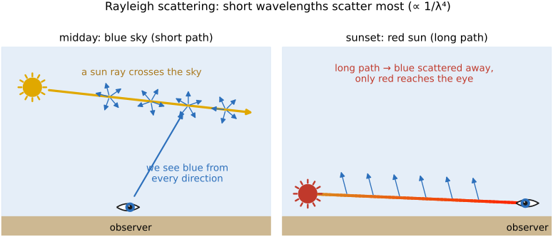
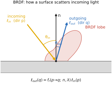
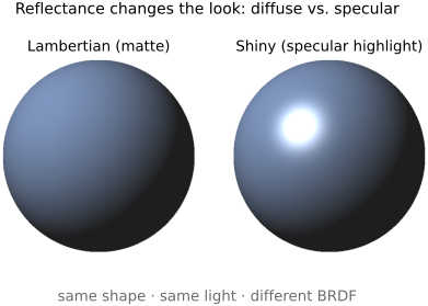
• **Light and physics** — what light *is* (wave / ray / photon), how it interacts with matter (reflection, refraction, scattering, the BRDF), and how we *measure* it (radiometry: radiance, irradiance, the inverse-square and cosine laws).
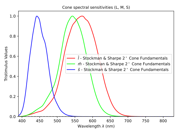
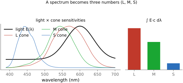
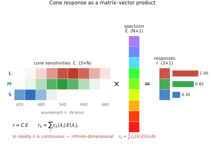
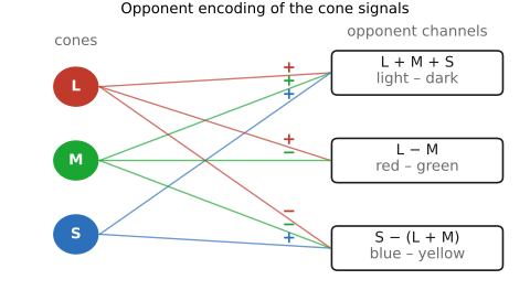
• **Human perception and color** — the eye and visual system; why three **cones** make us trichromatic; color as the projection of a spectrum onto three numbers; opponent processing, constancy, and the contrast sensitivity function. *(Placed early, right after light, because color is made in the observer and grounds everything downstream — encoding, white balance, JPEG, tone mapping.)*
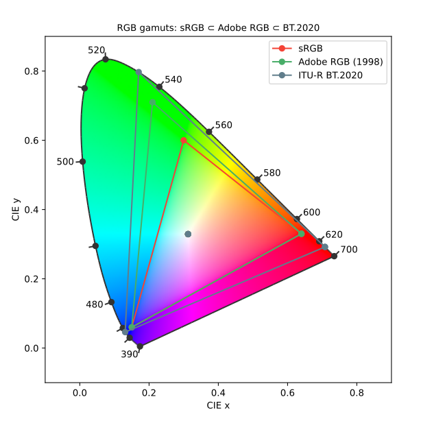
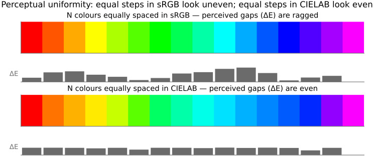
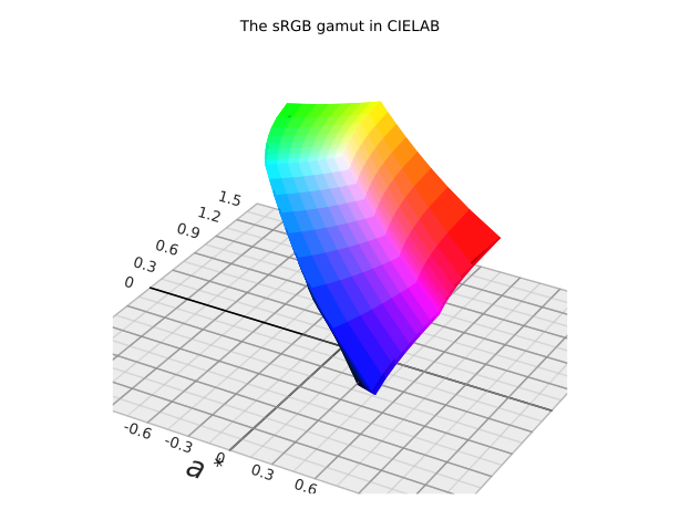
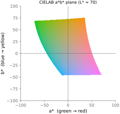
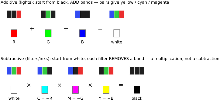
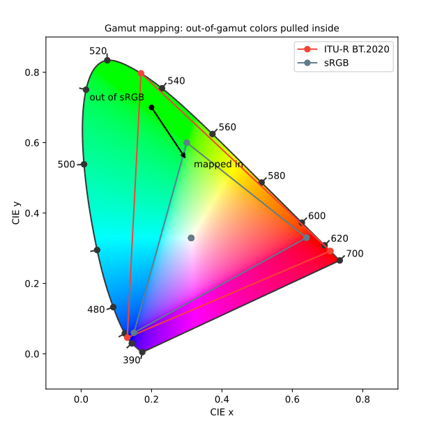
• **Measuring and encoding color** — the engineering payoff: **measuring** color (CIE), **encoding** it (linear / gamma / log, color spaces, CIELAB), and **reproducing** it (additive vs subtractive synthesis, gamuts, white balance, color management).
• **Image formation and linear perspective** — how a lens turns 3-D rays into a 2-D image (pinhole, perspective projection), depth of field, the **sensor** and the exposure triangle, **noise**, and the abstract framing the book leans on: imaging as a **linear system** and as an **inverse problem**.
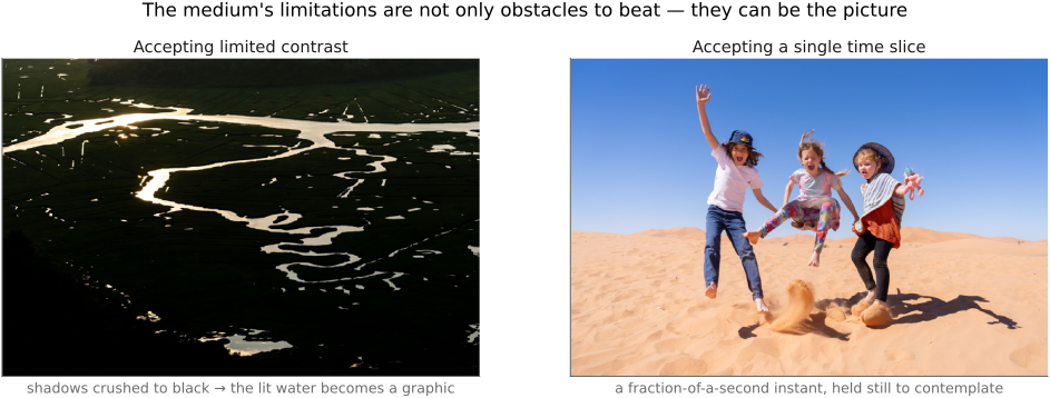
• **The limits of the medium** — having built the camera and the image from physics, step back and ask what a picture fundamentally cannot do: it is flat, framed, single-viewpoint, static, and limited in contrast and gamut, while the world and the eye are none of these. (The camera as an instrument and the question of photographic objectivity move to the next part, [[Photography]].)
• **skippable, but foundational**: a reader who only wants to code can jump straight to BASIC IMAGE PROCESSING — but the **big lessons** of this part recur everywhere later. The ones to carry forward:
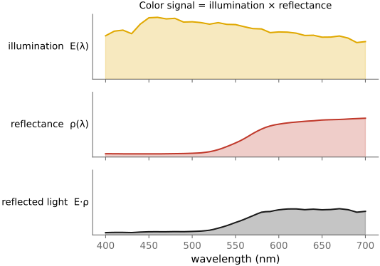
• **multiplicative vs additive** — much of imaging is *multiplicative* (illumination × albedo, contrast), some *additive* (incoherent light from different sources, blur); the right **encoding** (linear / log / gamma) follows from which one you are doing (→ [[Big Lessons]]).
• **gamma / ratios matter** — perception is roughly logarithmic, so we store images **gamma-encoded** to spend code levels where the eye looks; what matters is *ratios*, not absolute values.
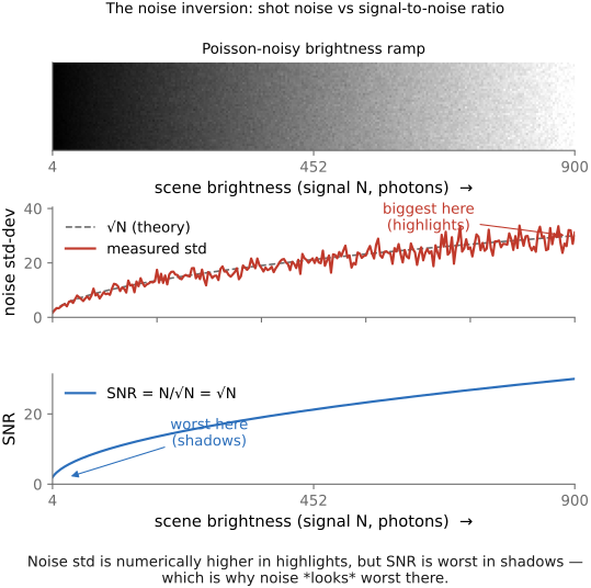
• **noise is affine** — sensor noise is **read + shot** (a constant plus a term that grows with the signal); because shot noise is **Poisson**, SNR is worst in the **shadows**, which is exactly where noise *looks* worst.
• **projective geometry is matrices + a division** — perspective projection is a **linear map in homogeneous coordinates** followed by a divide-by-depth; that single trick handles cameras, warps, and stereo.
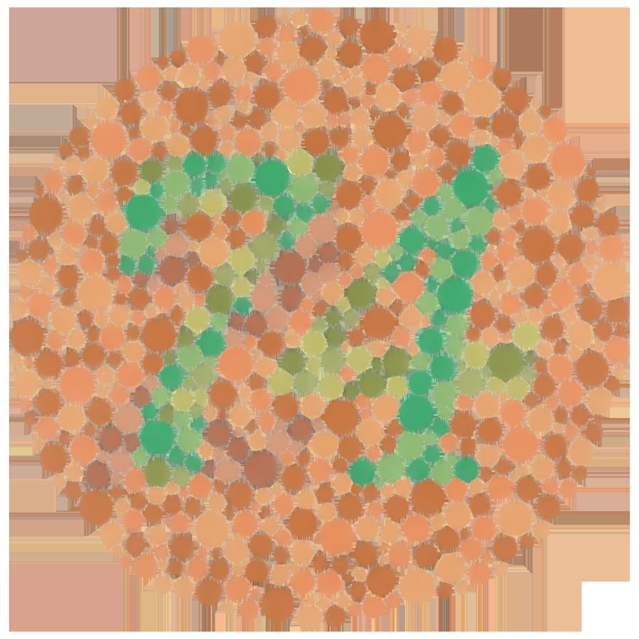
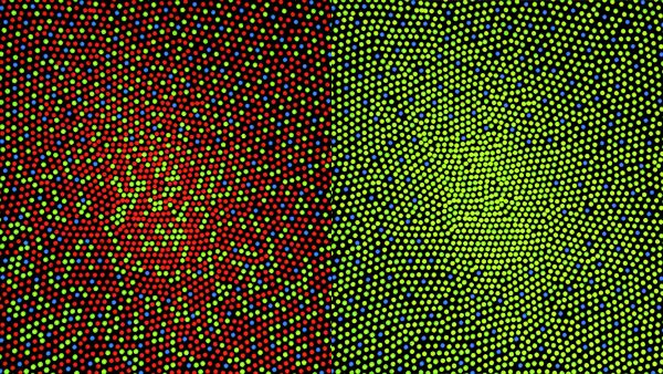
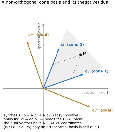
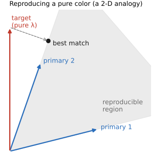
• **color is non-orthogonal and non-negative** — the cone "axes" overlap and light cannot be negative, which is what makes color sensing and reproduction genuinely hard (no perfect set of primaries; white balance is never exact).
• **by the end of this part** you can trace a photon from a lamp to a perceived color, reason quantitatively about exposure and noise, and you will carry the small set of principles the rest of the book keeps reusing.
2.1 Light and physics
• chapter intro: a working model of light — its **color** (spectrum), its **interaction with surfaces**, and its **energy** (radiometry); closes with the **plenoptic function** that ties the pipeline together
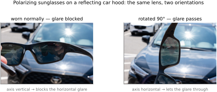
2.1.3 Polarization
2.2 Perceptual color and trichromatic vision
2.3 Human Vision
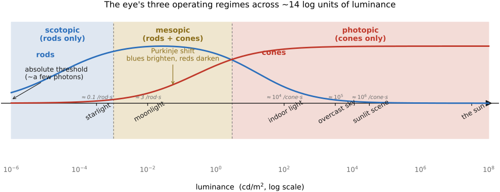
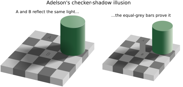
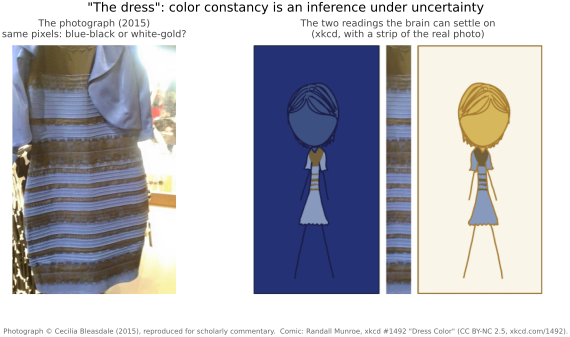
• the perceptual machinery the visual system runs *on top of* color: adapting to level, discounting the illuminant to report surface reflectance (constancy), working in ratios (contrast), and resolving detail unevenly across spatial/temporal frequency (the CSFs) — the properties compression, tone mapping, and display design optimize for.
2.4 Animal eyes
fig-eye-evolution
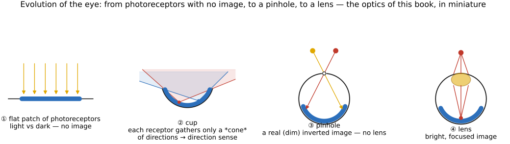
fig-eye-evolution · the evolution of the eye, in cross-sections: flat photoreceptor patch (no image) → cup (directional) → pinhole (an image, no lens) → lensed eye — recapitulating sensor → camera-obscura → lens (Bonus: animal eyes) 🟨
• **the eye evolved as a sequence of small improvements**, and it recapitulates the optics of this book — from "no image" to a focused one. Following Nilsson's stages (Land & Nilsson, *Animal Eyes*):
• **a flat patch of photoreceptors** (an *eyespot*): just **photosites**, **no image formation** — it tells light from dark and, crudely, which side has *more* light (phototaxis), but cannot form a picture. This is the bare **sensor** with no optics.
• **a concavity / cup**: fold the patch into a **pit** and the rim's shading gives **directional** sensitivity — the deeper the cup, the better you can tell *where* light comes from.
• **a pinhole**: close the cup almost shut → a **pinhole eye**, a real (if dim) **image** with no lens at all (the **nautilus** still uses one) — exactly the camera obscura of [[#Pinhole image formation and linear perspective]].
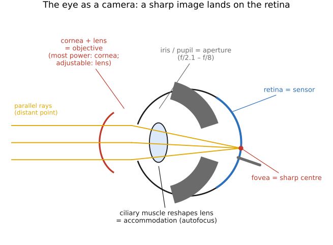
• **a lens**: fill the aperture with a **refractive lens** (often a graded-index sphere) → a **bright, focused** image, independently evolved in fish, cephalopods, and vertebrates. Add a **cornea, iris, and accommodation** and you have the human eye.
• so the human eye is *one* solution; evolution reached the same goal by very different routes (below).
• **a tour of those other solutions** — a useful contrast to the human eye and to camera design:
• **compound eyes** (insects): many **ommatidia** → wide field of view and fast temporal response, but low spatial resolution
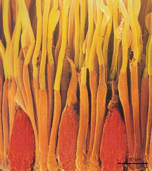
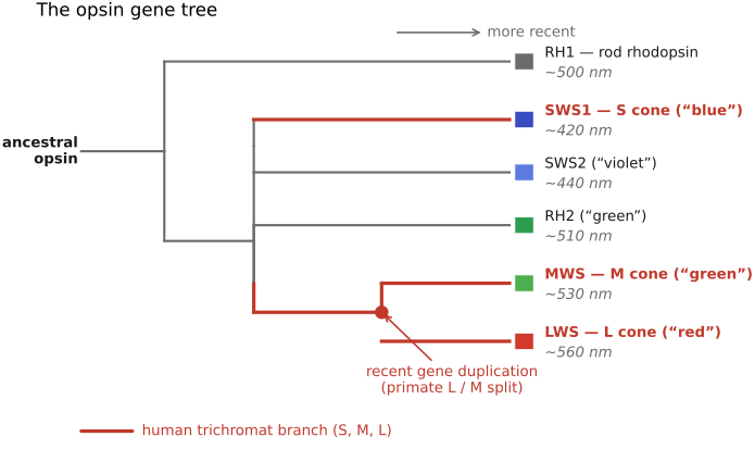
• **more cone types**: birds / reptiles are **tetrachromatic** (a 4th cone, into the UV); the **mantis shrimp** has ~12–16 photoreceptor classes (yet poor color *discrimination* — it seems to recognize rather than compare) — the **divergence of opsins** across animal groups is the color sidebar in [[#Color]]
• **tapetum lucidum** (cats, deer): a reflective layer behind the retina that boosts night vision (and causes eye-shine)
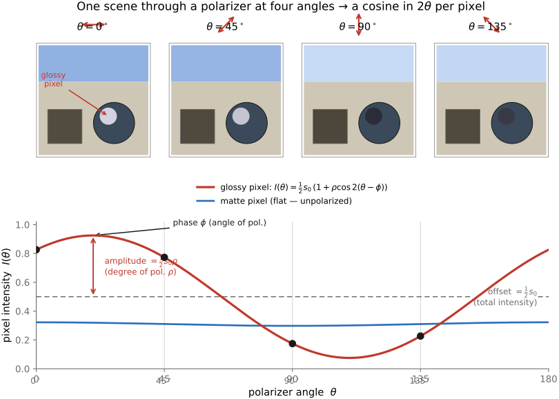
• **polarization vision** (cephalopods, many insects): they see light's **polarization** — a channel we're blind to
• **other eye designs**: **pinhole** (nautilus), **mirror eyes** (scallops — image formed by a concave mirror, not a lens), and the front-facing (**stereo**) vs side-facing (**field-of-view**) placement trade-off
• further reading: Land & Nilsson, *Animal Eyes*; the "Evolution of Eyes" chapter in *Vision* (Cambridge); a friendly overview at phos.co.uk, "The Evolution of Sight".
2.4.1 The optics: many ways to form an image
2.4.2 The color vision: opsins remixed
2.5 Measuring and encoding color
2.6 Pinhole image formation and linear perspective
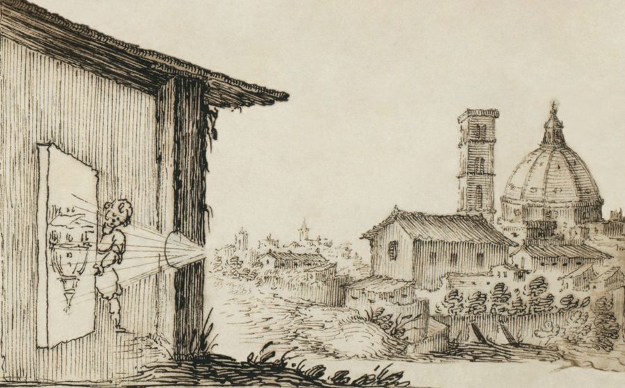
fig-camera-obscura
fig-camera-obscura · camera obscura / pinhole (artist's) 🟨
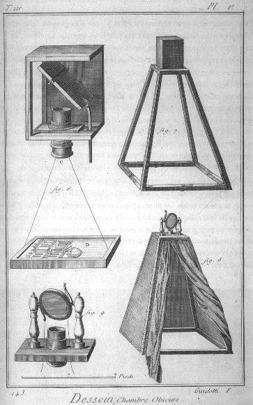
fig-camera-obscura-apparatus
fig-camera-obscura-apparatus · camera obscura apparatus (Diderot engraving) 🟨
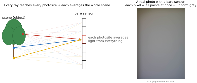
fig-bare-sensor-averaging
fig-bare-sensor-averaging · a bare sensor averages all rays 🟨
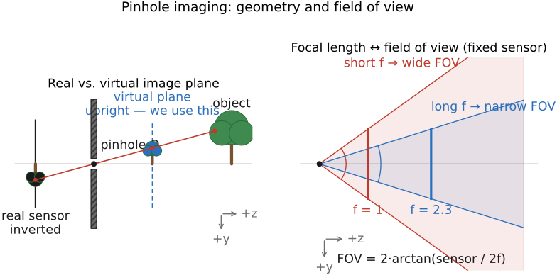
fig-pinhole-fov
fig-pinhole-fov · pinhole geometry: real (inverted) vs virtual (upright) image plane, and focal length → field of view 🟨
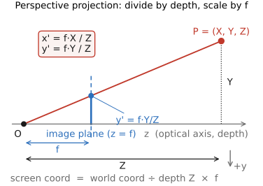
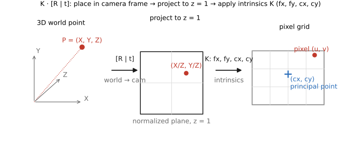
fig-perspective-projection
fig-perspective-projection · perspective projection equation: x'=f·X/Z, y'=f·Y/Z (divide by depth, scale by f) 🟨
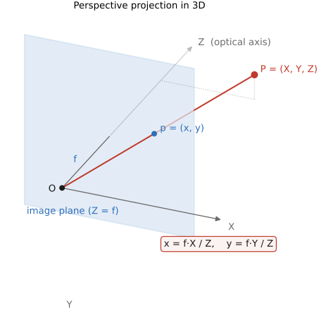
fig-perspective-projection-3d
fig-perspective-projection-3d · perspective projection in 3D: P=(X,Y,Z) → p=(x,y) on the image plane through the pinhole 🟨
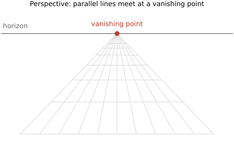
fig-perspective-vanishing-points
fig-perspective-vanishing-points · perspective projection + vanishing points 🟨
⬜ figure not yet created
focal length vs subject distance (background compression) fig-focal-length-compression
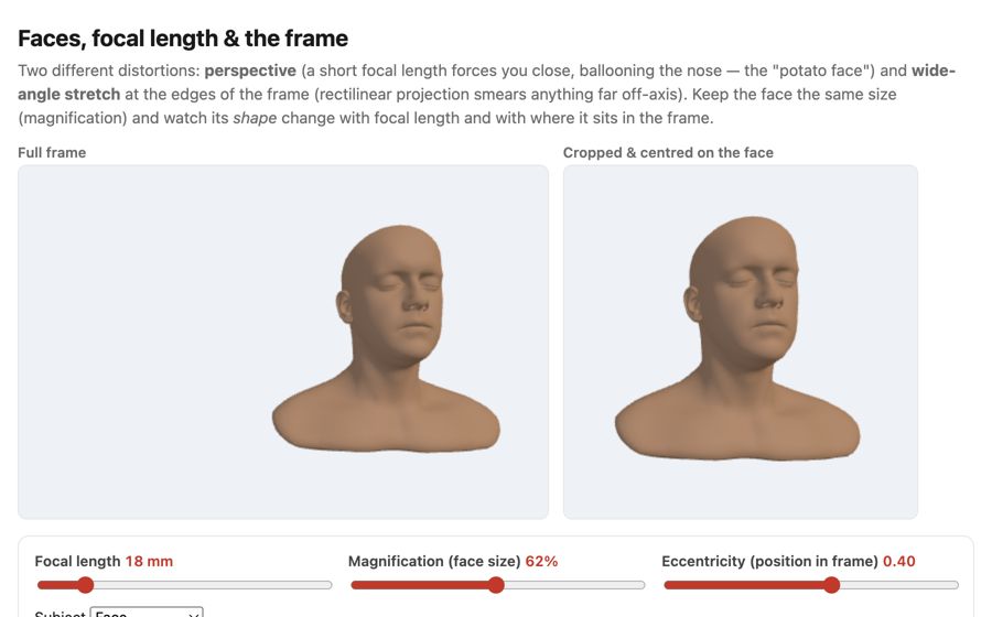
fig-face-distortion-sim
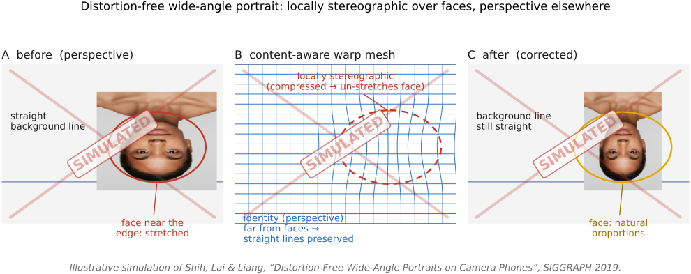
fig-face-distortion-sim · live face-distortion simulator (web edition): focal length + magnification + eccentricity controls with a full-frame view and a face-cropped view, showing the close-wide "big nose" perspective and the wide-angle edge stretch at constant face size; subject = a face, a grid sphere, or one of six diverse Meshy humans framed on the face; static fallback is a screenshot. *Human 3D models generated with Meshy AI.*
fig-dolly-zoom-sim
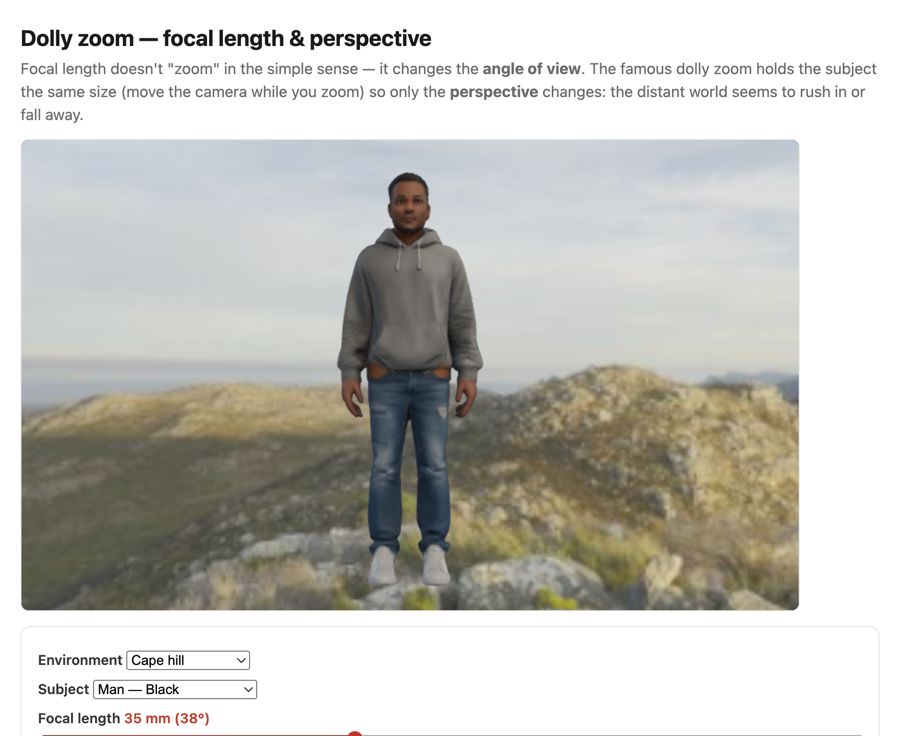
fig-dolly-zoom-sim · live dolly-zoom simulator (web edition): hold the subject size while focal length and camera distance trade off so only perspective / background scale changes; log focal (12–200 mm) + distance sliders, realistic Poly Haven environments, subject = head bust or one of six diverse Meshy humans. *Human 3D models generated with Meshy AI.*
fig-portrait-lighting-sim
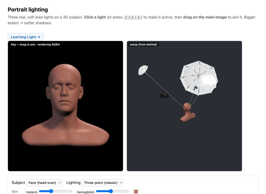
fig-portrait-lighting-sim · live portrait-lighting simulator (web edition): three soft area lights (key/fill/kicker — az/el/extent/intensity/colour, area-light-supersampled soft shadows) on a 3D face with a physiological melanin/hemoglobin skin model; a from-behind setup view with Meshy studio umbrellas + a camera rig; lighting presets; static fallback is a screenshot. *3D umbrella generated with Meshy AI.*
fig-keystoning-cause
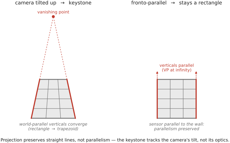
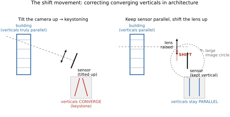
fig-keystoning-cause · keystoning is the tilt, not the lens — a camera tilted up makes world-parallel verticals converge (façade → trapezoid), while the fronto-parallel shot keeps them parallel; projection preserves lines, not parallelism 🟨
fig-point-line-duality
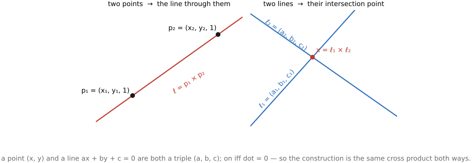
fig-point-line-duality · point↔line duality in homogeneous 2D: two points → a line, two lines → a point (same cross product) 🟨
fig-projection-decomposition
fig-projection-decomposition · projection-matrix decomposition K·[R matplotlib, 3-stage pipeline
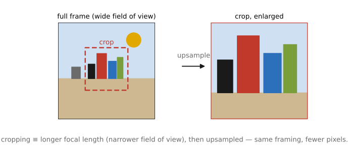
fig-crop-focal-length
fig-crop-focal-length · cropping = changing focal length: full frame vs a crop box ≡ a longer-focal-length capture, upsampled 🟨
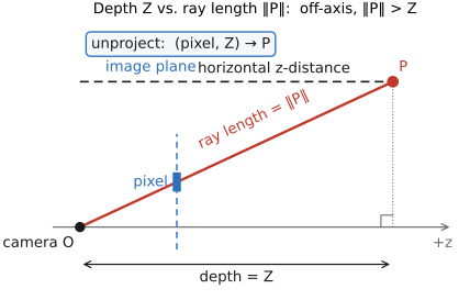
fig-depth-vs-ray-length
fig-depth-vs-ray-length · depth (z coordinate) vs ray length ‖P‖ from camera to a 3D point; unproject (pixel + depth → 3D) 🟨
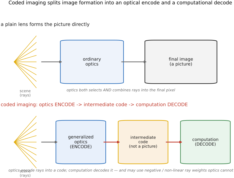
• sensor alone would capture a diffuse light. We need to select which rays from which part of the scene contribute to which pixel.
equations
pinhole projection x = f·X/Z, y = f·Y/Z
homogeneous p ≈ K·[R|t]·P
field of view = 2·arctan(sensor / 2f)
2.6.3 Camera in a general configuration
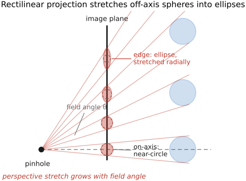
2.6.7 Wide-angle distortion: spheres bulge and faces stretch at the edges
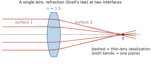
2.7 Lens image formation
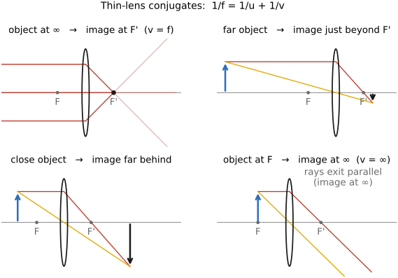
• chapter intro: from the **pinhole** (sharp but dim) to a **lens** (bright but with one focus plane) — refraction at curved surfaces, the thin-lens linearization, and the depth-of-field that the finite aperture forces on us
2.8 Image measurements as integrals
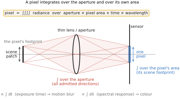
• chapter intro: the unifying idea behind sensing — **measurement = integrating a slice of the plenoptic function** — then the physical sensor that does it (photosites, CCD/CMOS) and the **noise** that limits it
• sidebar — **photography as objective measurement**: the medium's long arc bends toward objective measurement (film/print = a *performance*; → measurement). The **digital sensor** is the far end: because each photosite *counts photons*, a **raw** image is ≈ a **calibrated radiometric measurement** — a physical map of scene radiance, in real units, of one snapshot of time — not just a rendering. This is what makes HDR / depth / deblur possible: the pixel numbers must *mean* something physical. Ties to the intro's **generation → measurement → generation** arc (→ [[01 Intro]]).
2.8.3 Splitting the integral
2.9 Depth of field
fig-circle-of-confusion
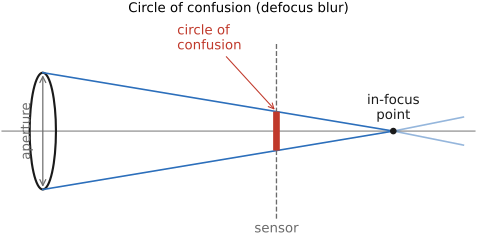
fig-circle-of-confusion · finite aperture & circle of confusion
fig-defocus-vs-parameters
fig-defocus-vs-parameters · defocus blur (CoC) vs aperture and object distance 🟨
fig-depth-of-field
fig-depth-of-field · near/far limits where blur reaches c (linearized DoF) 🟨
fig-dof-derivation-near
fig-dof-derivation-near · near (front) limit by similar triangles — all quantities 🟨
fig-dof-derivation-far
fig-dof-derivation-far · far (back) limit by similar triangles — all quantities 🟨
fig-dof-vs-parameters
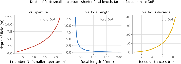
fig-dof-vs-parameters · DoF vs aperture, focal length, focus distance 🟨
fig-hyperfocal
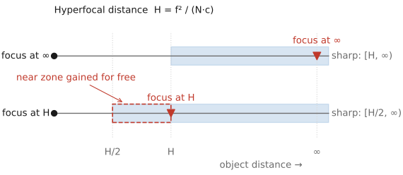
fig-hyperfocal · hyperfocal: focus at H → sharp from H/2 to ∞ 🟨
fig-dof-same-framing
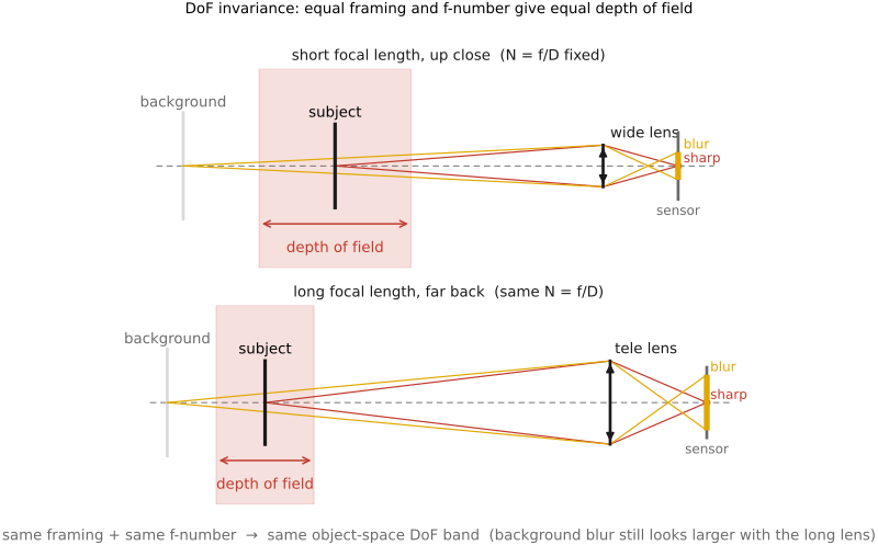
fig-dof-same-framing · same framing + same f-number → same object-space DoF (short vs long focal length); background blur still looks larger with the long lens 🟨
fig-dof-double-cone
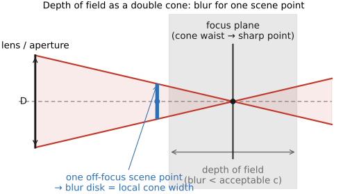
fig-dof-double-cone · object-space DoF as a double cone in front of the lens, waist on the focus plane (the blur for one scene point) 🟨
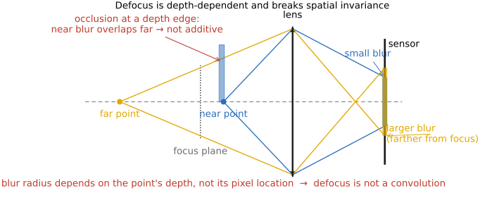
fig-dof-depth-dependent
fig-dof-depth-dependent · defocus is NOT a convolution: blur radius depends on scene depth (not pixel location), and occlusion at depth edges 🟨
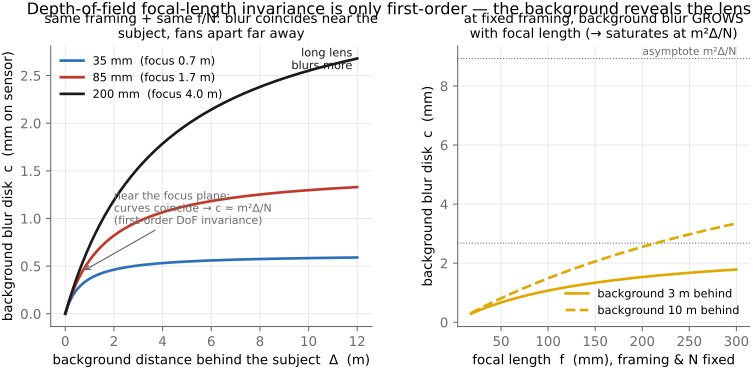
fig-dof-background-blur
fig-dof-background-blur · DoF focal-length invariance is only first-order: background blur c vs background distance for 35/85/200 mm (matched framing & N) coincide near the subject and fan apart far away; + c vs focal length showing growth/saturation
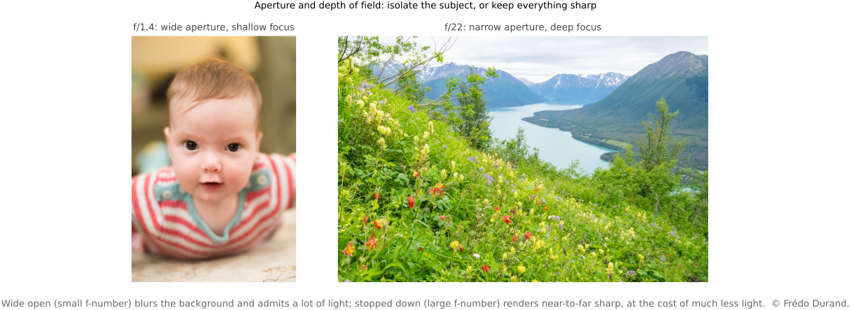
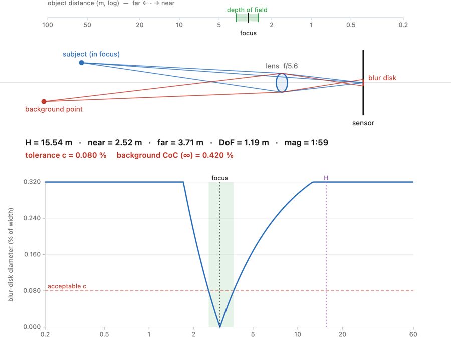
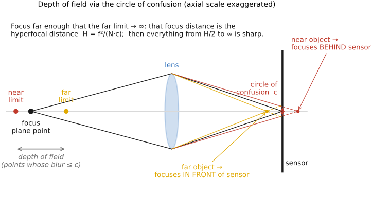
• **defocus / circle of confusion**: a point off the focus plane images to a point that is not on the sensor, so the aperture cone meets the sensor as a blur disk — the **circle of confusion**. A point still counts as sharp while its disk stays within an acceptable c. [CoC figure]
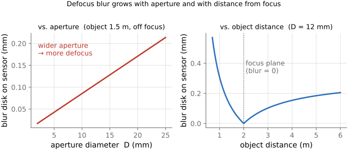
• the blur disk grows with the **aperture** (wider → bigger disk) and with the **object's distance from the focus plane** (zero exactly at focus); focal length and focus distance enter too. [defocus-vs-parameters figure]
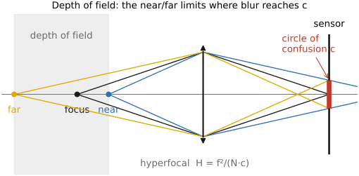
• **depth of field** = the *range* of object distances whose blur disk stays within c; the **near** and **far** limits are where the blur just reaches c. [DoF near/far figure — each cone carried out to the CoC at the sensor]
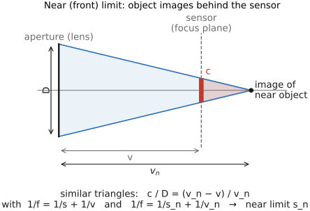
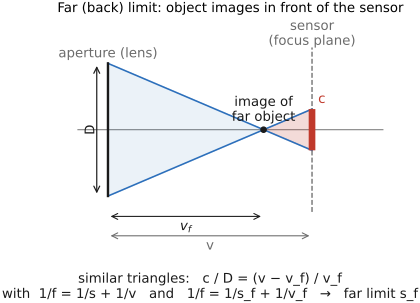
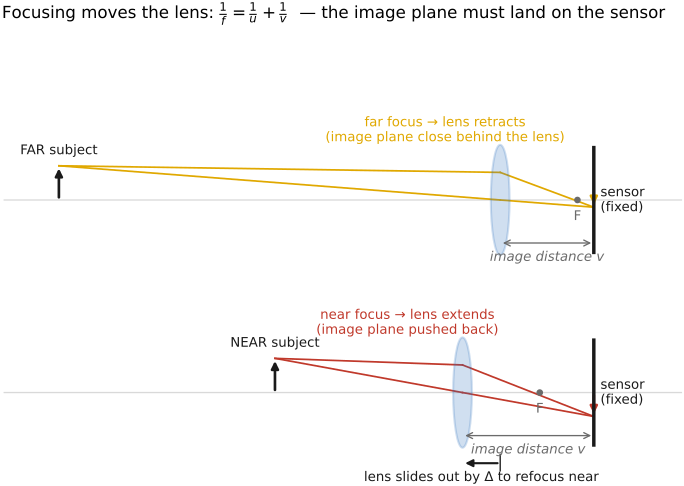
• **deriving the limits**: on the image side a near-limit object images *behind* the sensor and a far-limit object *in front* of it; **similar triangles** relate the aperture D, that convergence distance, and the circle of confusion c — and together with the conjugate relations (1/f = 1/s + 1/v) they fix the near (front) and far (back) object-distance limits. [near-limit and far-limit similar-triangle figures]
• **hyperfocal distance** H = f²/(N·c): focus there and everything from **H/2 to infinity** is acceptably sharp — the focus setting that maximizes DoF (focusing at ∞ instead wastes the H/2…H zone). [hyperfocal figure]
• DoF **grows** with a smaller aperture (larger N), a shorter focal length, and a greater focus distance — these are the paraxial (linearized) formulas; the accurate model is in the Optics part. [DoF-vs-parameters figure]
• **the surprising invariance** (the lecture's flagged "important conclusion"): for a **fixed framing** (same subject size) and a **fixed f-number**, the depth of field in **object space** is essentially **independent of focal length** — switching 28 mm → 100 mm forces you to step back, and the larger physical aperture cancels the longer focal length. So "long lenses have shallow DoF" is really about **magnification**, not focal length per se. (The *background* still looks more blurred with the long lens — that's magnification of the out-of-focus disk, not a DoF change.) [same-framing/same-N → same DoF figure]
• ⚠️ **but the invariance is only *first-order* — the background gives the focal length away.** "Same framing + same f-number → same DoF" is the **small-defocus (paraxial)** result: it holds for the **near/far acceptable-sharpness limits straddling the subject**, but **not** for how hard a *distant* background is thrown out of focus. **Derivation** (thin lens; blur-disk diameter on the sensor): a point at distance $s_b$, with the lens focused at $s_f$, images to a circle of confusion $c \approx \dfrac{f^2}{N}\,\dfrac{|s_b-s_f|}{s_b\,s_f}$. **Fix the framing** — subject magnification $m=f/s_f$ held constant, so $s_f=f/m$ — and **fix $N$**, with the background a gap $\Delta=s_b-s_f$ behind the subject:
$$c(f)=\frac{m^2\Delta/N}{\,1+ m\Delta/f\,}\ \xrightarrow[f\to\infty]{}\ \frac{m^2\Delta}{N}.$$
The subject-zone DoF is ~independent of $f$ (the leading $f$ cancels — the **first-order invariance**), but the **background blur grows monotonically with focal length**, saturating at $m^2\Delta/N$. Two shots matched in framing *and* aperture render the **subject** identically, yet a **200 mm melts a far background far more** than a 35 mm: the correction term is order $m\Delta/f$ — negligible for a background near the focus plane (invariance looks exact), but dominant once the background is many focus-distances away. This is exactly why portrait shooters reach for long lenses for "background separation" even though the DoF on the *face* is unchanged. **Full derivation + plots** of $c$ vs. background distance for 35 / 85 / 200 mm (fixed framing & $N$) — the curves coincide near the focus plane and fan apart far from it. [`fig-dof-background-blur`]
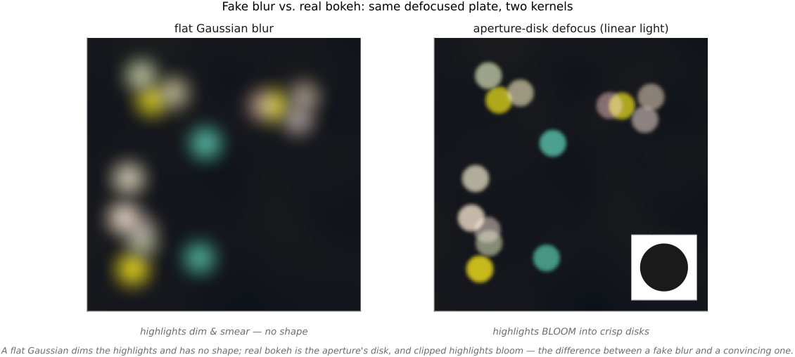
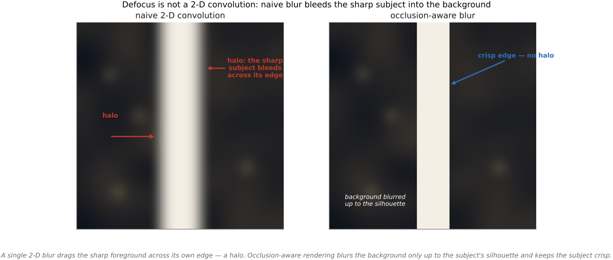
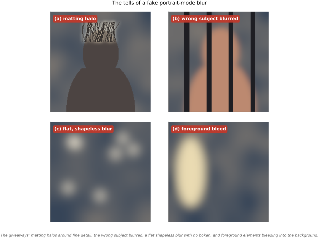
• **object-space picture & a caveat**: the simplest view is a **double cone** in front of the lens whose waist sits on the focus plane — it gives the blur for **one** scene point. But **defocus is *not* a spatially-invariant convolution**: the circle of confusion depends on each point's **scene depth** (not its pixel location), and at depth discontinuities **occlusion** matters — which is why naive "just blur the image" fakes look wrong, and why light-field / depth-aware methods (Advanced) do better. [object-space double cone; depth-dependent-blur + occlusion figure]
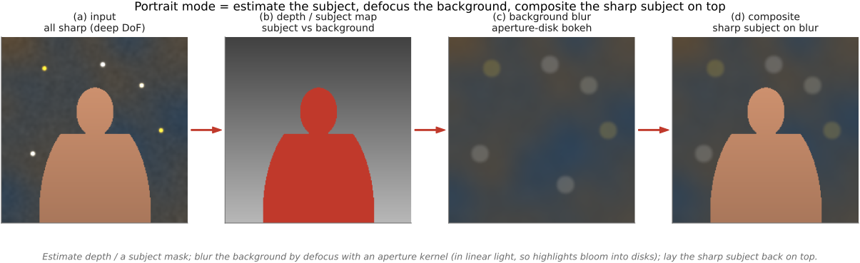
• **sensor size scales DoF**: shrink the sensor (keeping FOV) and both the circle of confusion and the aperture shrink, so DoF grows **linearly** with sensor size — why phone cameras have huge DoF (and resort to *computational* background blur), and why **macro is easier on small sensors** (a scaled-down camera photographs a scaled-down world — modulo diffraction)
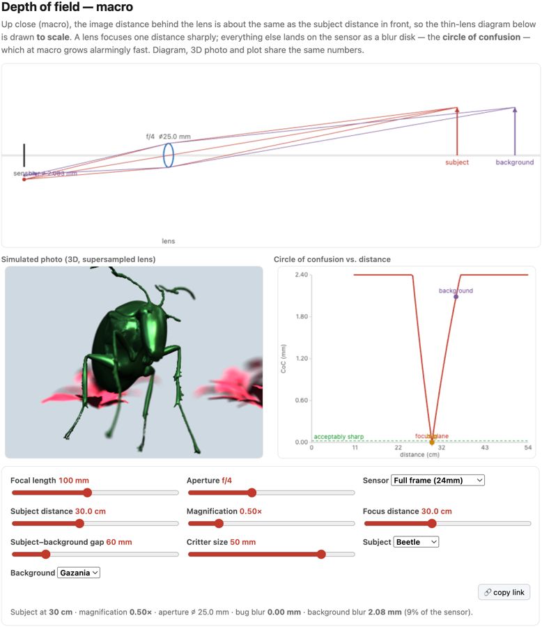
• 🖱️ **Interactive (web edition):** a live **macro depth-of-field simulator** — a to-scale thin-lens diagram, a lens-supersampled 3D photo (real bokeh), and a circle-of-confusion-vs-distance plot all driven by one shared optics model (focal length, f-number, sensor, focus distance, subject–background gap). A 3D bug (beetle / bee / ladybug) over a flower makes the macro lesson vivid: focus lands on the front of the face and the rest of the body, antennae, and background all fall out of focus. [fig-depth-of-field-sim; interactive] *(bug & flower 3D models generated with Meshy AI — acknowledge in the caption)*
equations
acceptable blur = circle of confusion c
defocus blur diameter b = D·|v − v′|/v′
hyperfocal H = f²/(N·c)
near limit D_n = s(H−f)/(H+s−2f)
far limit D_f = s(H−f)/(H−s)
total DoF = D_f − D_n
2.10 Motion blur
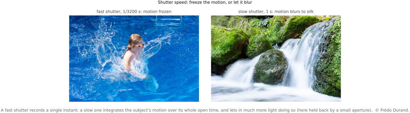
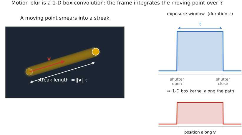
• **blur from subject motion**: $b_{px}\approx f_{px}\,v\Delta t/D$ — a straight streak = image velocity × exposure (constant-velocity linearization); only cross-axis motion blurs
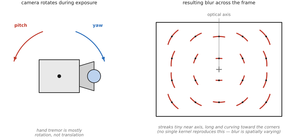
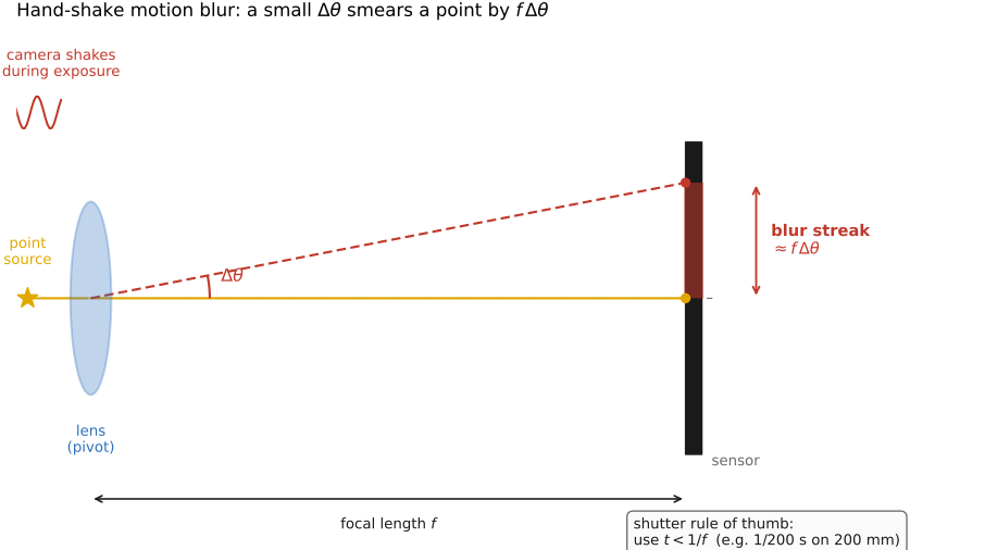
• **blur from camera shake**: translation $b\approx f_{px}\Delta_c/D$ (depth-dependent); rotation yaw/pitch $b\approx f_{px}\theta$ (**depth-independent**, small-angle); roll = spin about centre, grows with radius
• **which dominates**: ratio $\theta D/\Delta_c$ → rotation wins at normal distance, translation only up close (macro); rotation blur is **spatially non-uniform** so one kernel can't undo it (Whyte); IMUs measure the rotation to deblur (Joshi)
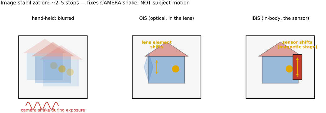
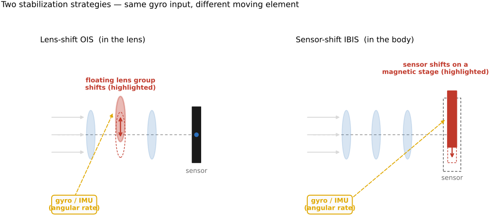
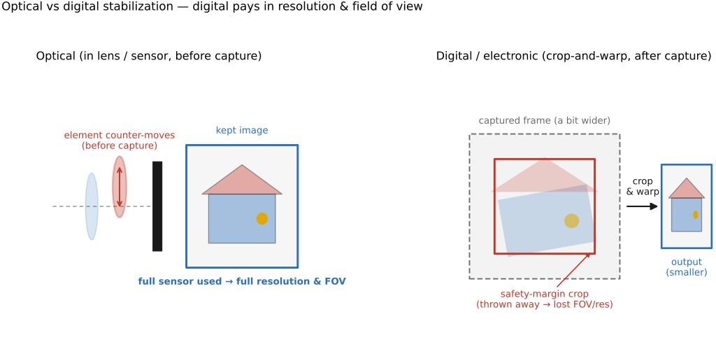
• **hand-holding rule** $\Delta t\lesssim 1/f$ s (×crop; ~2× faster for dense sensors); **image stabilization** cancels camera *rotation* (buys 3–5 stops) but not *subject* motion
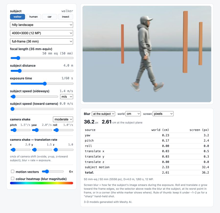
• 🖱️ **Interactive:** motion-blur calculator — 3-D scene (Meshy walking human / car), temporal-supersampled blur, world+screen readout by source, motion-vector & flow-colour overlays, hover pixel scale [fig-motion-blur-calculator; interactive]
2.11 Sensors: photosites, CCD vs CMOS
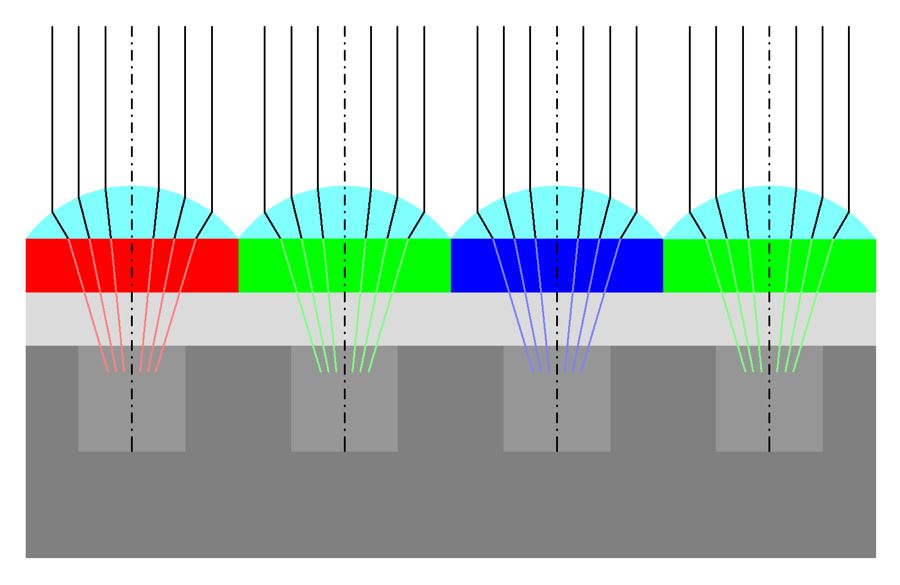
fig-sensor-microlens
fig-sensor-microlens · sensor cross-section: microlens → filter → photosite 🟨
⬜ figure not yet created
CCD bucket-brigade readout vs CMOS read-in-place schematic fig-ccd-vs-cmos
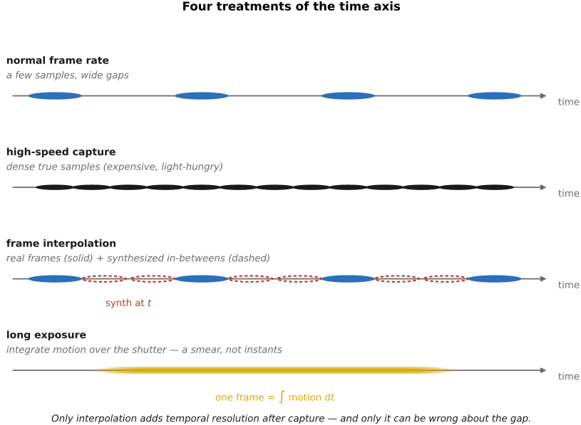
fig-slowmo-axis
fig-slowmo-axis · four ways to treat the time axis on a shared timeline — normal capture (sparse), high-speed (dense true samples), interpolation (sparse reals with synthesized in-betweens), and long-exposure blur (the integral); only interpolation adds resolution after capture and can be wrong 🟨
fig-mirrorless-anatomy
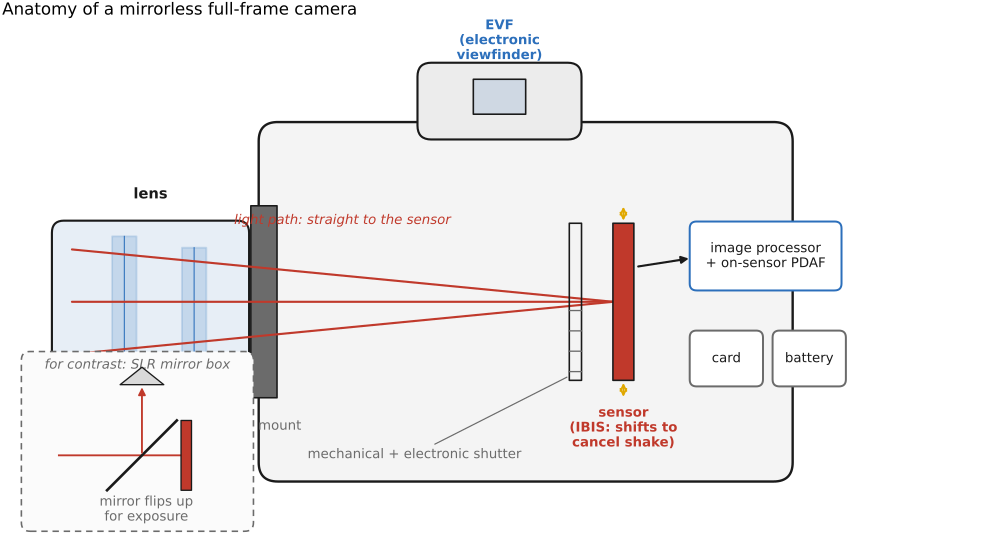
fig-mirrorless-anatomy · labeled cutaway of a mirrorless full-frame camera (lens+mount, sensor/IBIS, mech+electronic shutter, EVF, processor/on-sensor PDAF, card+battery); SLR mirror-box inset for contrast
fig-rolling-shutter
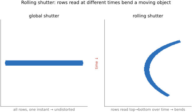
fig-rolling-shutter ·
fig-flash-sync
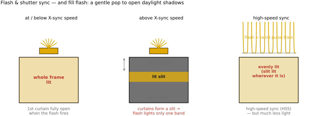
fig-flash-sync · flash & focal-plane-shutter sync: whole frame ≤ X-sync · slit/partial frame above it · high-speed-sync pulse train; fill-flash noted
fig-lippmann
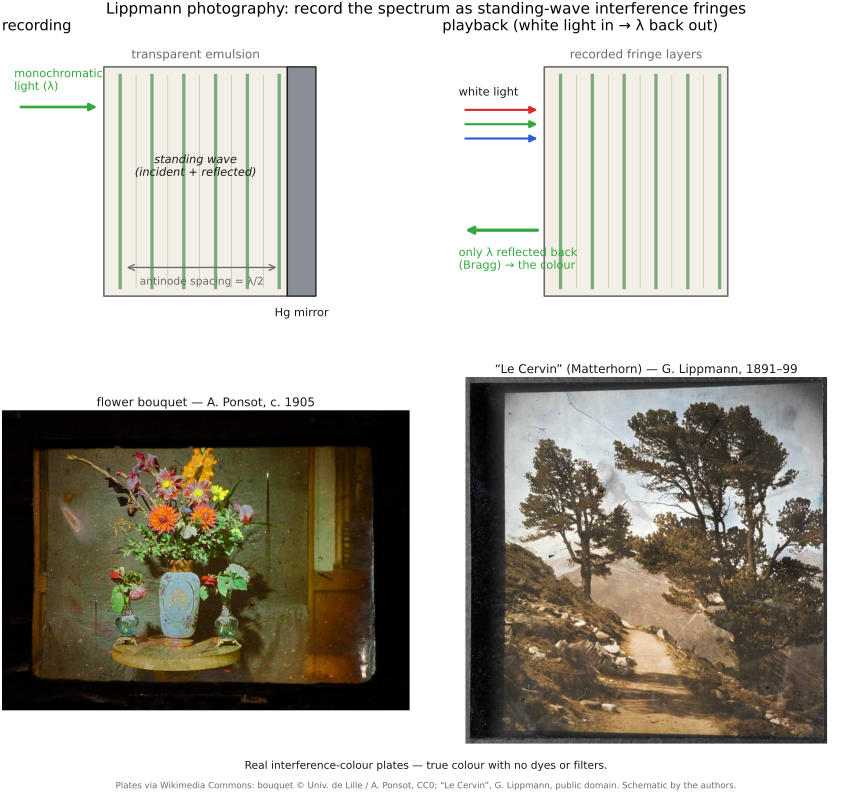
fig-lippmann · Lippmann interference colour photography: recording (standing wave in a mercury-backed emulsion, antinodes λ/2 apart) + playback (Bragg reflection of the original wavelength under white light)
2.11.3 Analog-to-digital conversion
2.11.6 Shutters
2.11.10 The impact of sensor size
2.11.11 How far sensors have come
2.12 Sensing color: multiplexing strategies
fig-color-multiplexing
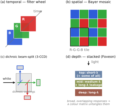
fig-color-multiplexing · four colour-sensing multiplexing strategies: temporal, spatial (Bayer), **dichroic 3-CCD** beam-split, depth (Foveon, with realistic broad/overlapping layer colours + colour-matrix note) 🟨
⬜ figure not yet created
temporal multiplexing artifact — Prokudin-Gorskii color fringes on moving water fig-prokudin-gorskii
• four ways to turn a monochrome sensor into a color one — **multiplex** the three (or more) measurements across some axis:
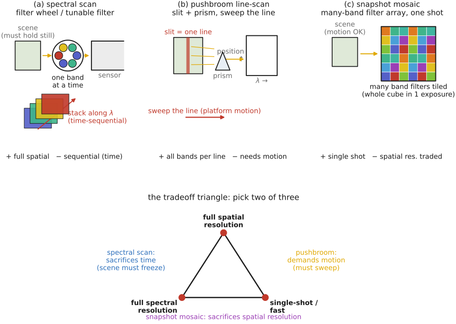
• **in time**: shoot R, G, B frames sequentially through filters — Maxwell's first color photograph (1861), **Prokudin-Gorskii**, flatbed scanners, astronomy filter wheels. Cheap and full-resolution, but **fails on motion** (the classic color fringes on moving water).
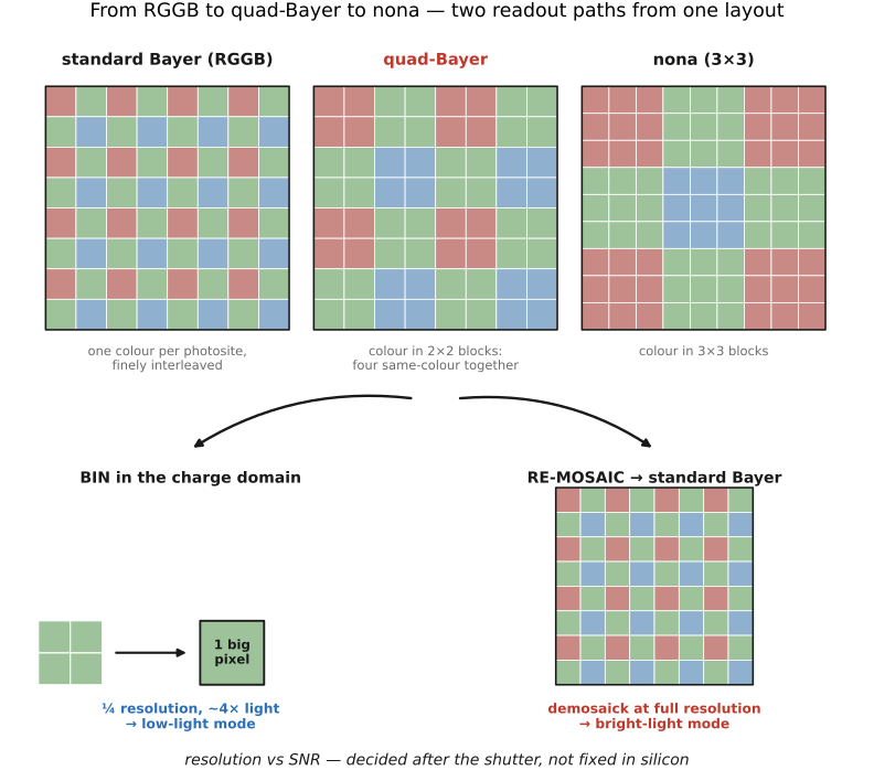
• **in space (the dominant choice)**: a **color filter array (CFA)** — the **Bayer mosaic** (2 green : 1 red : 1 blue) — one color per photosite, then **demosaick** to fill the rest; the eye does the same with its interleaved cone mosaic. Variants: Fuji's **X-Trans** (a larger, less-periodic tile to fight moiré) and **complementary CMY/CYGM** CFAs (more light through, messier color). Needs an **optical anti-aliasing (low-pass) filter** to tame high-frequency color artifacts, and suffers some channel **crosstalk**.
• **beam-splitter (prism)**: a **dichroic prism** splits the rays onto **three sensors** — **3-CCD / 3-chip**, the classic **broadcast video camera** — wasting no photons at full per-channel resolution, but bulky, costly, and hard to align.
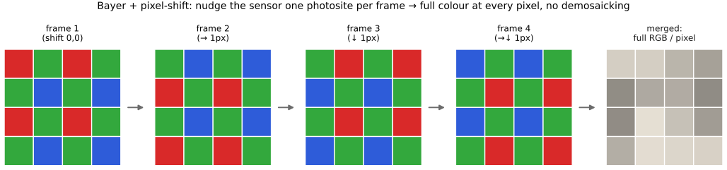
• **in depth (stacked)**: stack wavelength-selective layers so one location senses all three — **Foveon** (silicon absorbs longer wavelengths deeper; used in **Sigma** cameras), echoing **Kodachrome**'s stacked dye layers. Full color at every pixel (**no demosaicking**), but trickier color separation and more chroma noise.
• **spectral / Lippmann**: record the standing-wave **interference** of the full spectrum (Lippmann, 1908 Nobel; a precursor to holography) — true spectral capture, not just 3 numbers.
• **hybrid**: combine these (e.g. spatial + temporal in video).
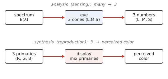
• this is *analysis* (sensing color) — the mirror of color *synthesis* (reproduction, above); the **demosaicking** algorithm itself is deferred to Basic Image Processing (which is why this is just the *sensing* half)
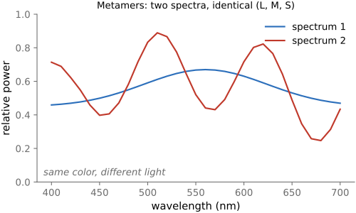
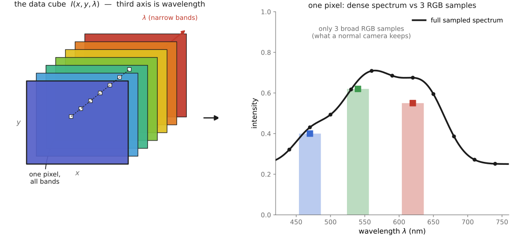
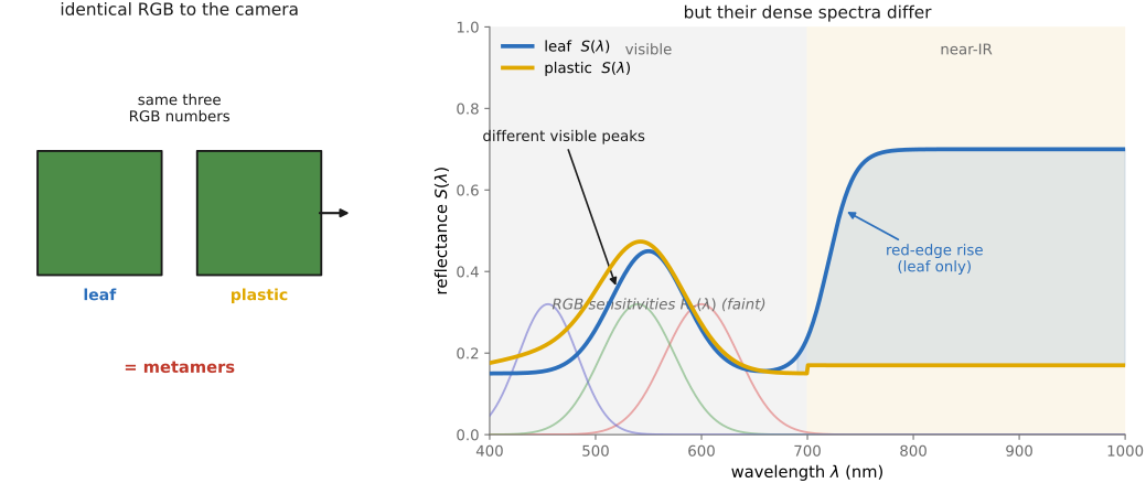
• **trichromatic (perceptual) vs spectral (physical) capture**: almost all imaging systems aim to capture **perceptual, trichromatic color** — three numbers that reproduce what a *human* would see (RGB ≈ the cones), so metamers are, by design, indistinguishable. **Multispectral / hyperspectral** imaging instead samples the **physical spectrum** in many narrow bands (tens to hundreds), keeping distinctions the eye throws away — for remote sensing, agriculture, art conservation, and machine vision, where the *material*, not the *appearance*, is what matters (and metamers must be told apart). Lippmann (above) is the limiting case: the full continuous spectrum.
2.13 Noise, signal-to-noise ratio and dynamic range
⬜ figure not yet created
noisy image + flat-patch histogram (ISO 3200) fig-noise-histogram
⬜ figure not yet created
noise vs ISO fig-noise-vs-iso
fig-noise-affine
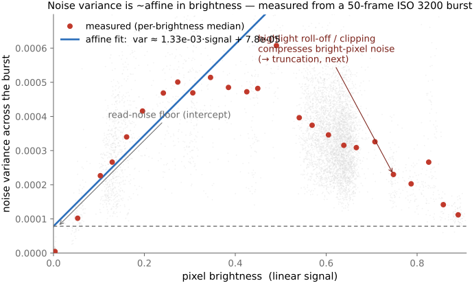
fig-noise-affine · measured noise variance is affine in brightness (σ²≈gain·I+read²) — real per-pixel variance vs mean from a 50-frame aligned ISO-3200 burst, with the affine fit, read-noise floor, and highlight roll-off (Noise, SNR, dynamic range)
fig-noise-gaussian-pixels
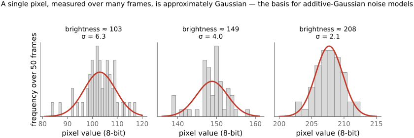
fig-noise-gaussian-pixels · a single pixel's value across many frames is ≈ Gaussian — per-pixel histograms from the ISO-3200 burst with Gaussian overlays (Noise)
fig-noise-truncation
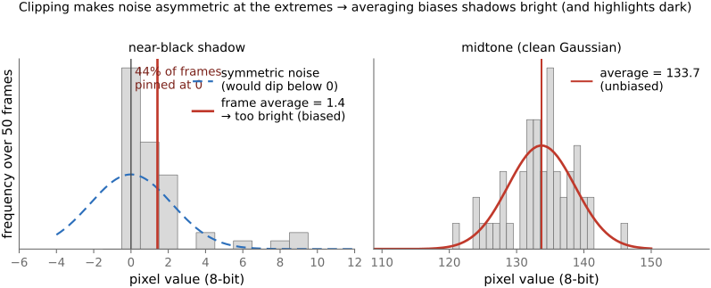
fig-noise-truncation · noise clips at black/white so it is not zero-mean at the extremes — a near-black pixel pinned at 0 ~44% of frames, its average biased bright, vs an unbiased midtone (Noise; denoising trap)
fig-snr-vs-stddev
fig-snr-vs-stddev · noise std-dev map vs SNR map of a brightness ramp: std rises with brightness (∝√N), but SNR=√N is worst in the shadows 🟨
⬜ figure not yet created
**underexposure recovery — full-frame vs phone**: the same underexposed scene pushed up several stops in software, the full-frame frame cleaning up while the phone reveals amplified shadow noise / banding [fig-underexposure-recovery-ff-vs-phone fig-underexposure-recovery-ff-vs-phone
fig-results-montage
fig-results-montage · a montage of computational-photography results — HDR tone mapping, refocus-after-capture, motion deblur, a stitched panorama — the "look what computation buys you" opener
fig-dynamic-range-comparison
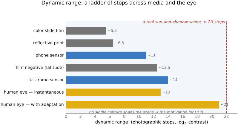
fig-dynamic-range-comparison · dynamic-range ladder in **stops** (horizontal bars): colour slide (~5–6) · reflective print (~6–7) · film negative (~12–13) · phone sensor (~10–12) · full-frame sensor (~14) · human eye instantaneous (~10–14) vs adapted (~20+) · an animal example · a typical sun-and-shadow scene (>20) — shows why no single capture holds a high-contrast scene (→ HDR)
⬜ figure not yet created
an animal or two
• the noise **sources** (their variances add):
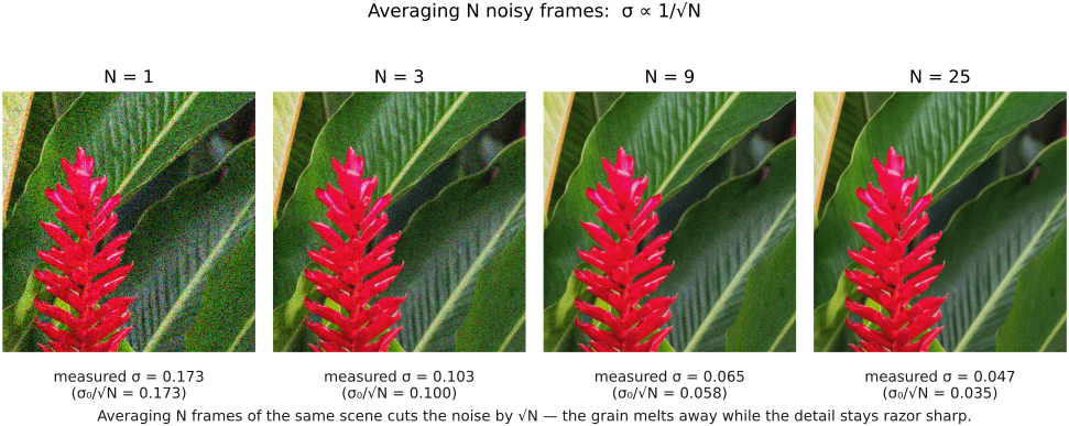
• **photon / shot noise** — the Poisson statistics of *counting photons*: variance = mean, so σ = √N. Fundamental (it's the light itself), dominates the midtones/highlights; averaging N independent frames cuts it by √N.
• **read noise** — added by the amplifier / ADC on readout; signal-independent, dominates the **shadows** and sets the noise floor (hence dynamic range).
• **thermal / dark current** — electrons freed by heat, independent of light; grows with exposure time and temperature (long exposures & astrophotography → sensor cooling, dark-frame subtraction).
• **fixed-pattern / pattern noise** — per-pixel gain/offset non-uniformity (PRNU/DSNU), hot/stuck pixels, banding; *structured*, so it reads as worse than random noise of equal magnitude, and is removed by calibration (flat / dark fields).
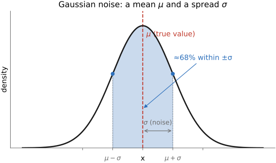
• 💡 **Big lesson — in a *linear* image, noise variance is an *affine* function of brightness.** The variances add: shot noise gives a term **proportional to the signal** (Poisson, variance = mean, scaled by the gain) and read noise a **constant** floor, so the total is **variance ≈ gain·signal + read²** — a straight line in brightness. You can *measure* it: take an aligned **burst** of a static scene and, per pixel, plot the variance across frames against the mean — the points trace that line, slope = photon gain, intercept = the read-noise floor. And a single pixel's value over many frames is **≈ Gaussian**, which is what licenses additive-Gaussian noise models. [`fig-noise-affine` — per-pixel variance vs brightness, measured from a 50-frame ISO-3200 burst; `fig-noise-gaussian-pixels` — per-pixel histograms] → register [[Big Lessons]]
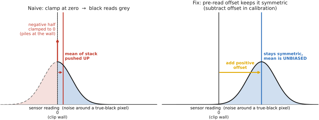
• 💡 **Big lesson — noise is *clipped* at black and white, so near the extremes it is *not* zero-mean.** A recorded value is clamped to [0, max]: near black the negative half of the noise is cut off (frames pile up at 0), near white the positive half is. So at the extremes the noise distribution is **asymmetric** and its mean is pushed **inward**. The consequence for **denoising**: any naive average/smoothing returns that biased mean, so it makes **shadows come out too bright and highlights too dark** — a bias every denoiser has to correct for (carried forward to [[#Denoising basics]] in BASIC). [`fig-noise-truncation` — a near-black pixel pinned at 0 a third of the time, its average biased bright; from the ISO-3200 burst] → register [[Big Lessons]]
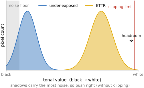
• **the key intuition — it's about ratios (SNR)**: shot noise is **Poisson**, so σ = √N grows with brightness — measured noise is actually **higher in the highlights**. Yet noise *looks* worst in the **shadows**, because perception cares about the **signal-to-noise ratio** SNR = N/√N = √N, which is worst where N is small. "Ratios are all that matters" — the same reason we encode in gamma/log, and the motivation for ETTR (below — Photography 101). [std-dev map vs SNR map figure]
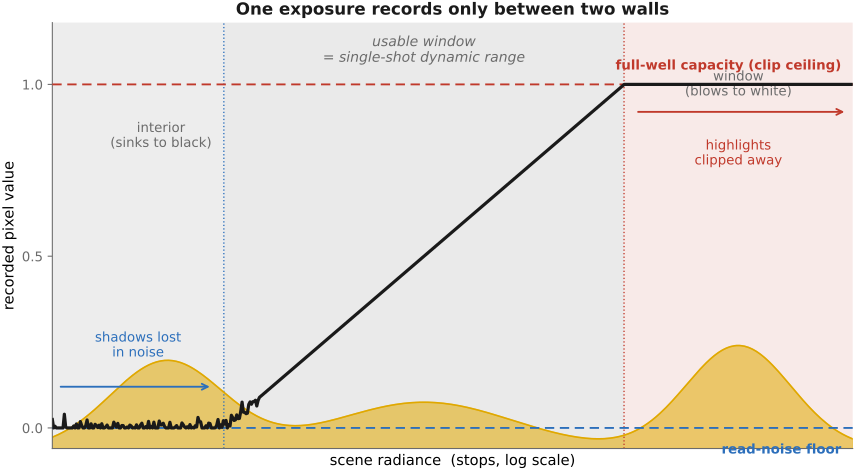
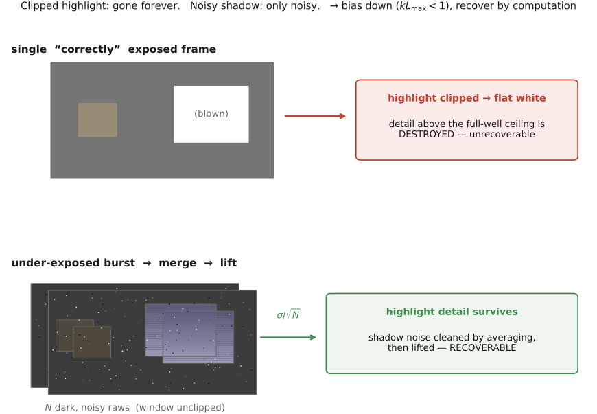
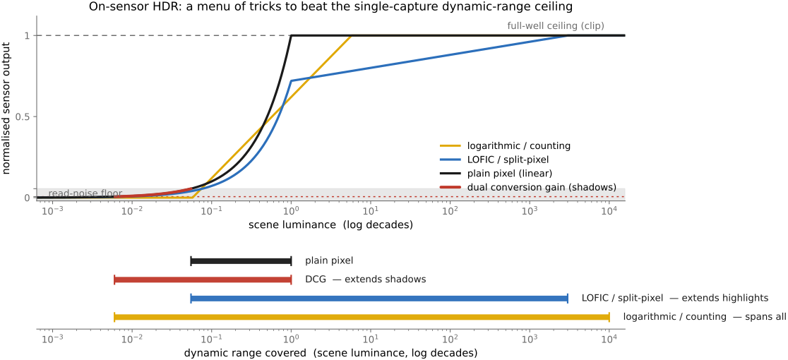
• **dynamic range** = the brightest recordable signal (sensor **saturation / full-well**) ÷ the **noise floor** (read noise in the shadows); it sets how much of a high-contrast scene fits in a *single* exposure → the motivation for **HDR** (Multiple exposure)
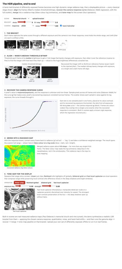
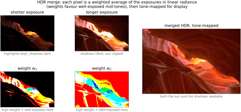
• **HDR (high dynamic range)**, sometimes called **wide dynamic range (WDR)**, is a deliberately **fuzzy** term — flag this. It gets used for at least four different things: the *scene* (a high-contrast world), the *capture* (multi-exposure / a high-DR sensor), the *file/encoding* (float or ≥10-bit radiance, e.g. OpenEXR, HDR10), and the *display* (an HDR monitor) — and, loosely, for the **tone-mapped "HDR look."** There is no single sharp definition; say which sense you mean. (Developed in [[Multiple exposure imaging]].)
• 💡 **Big lesson (L2.48) — dynamic range is set by full-well capacity over the noise floor**: a single exposure records from a **top** (the photosite's **full-well capacity** — where it clips to white) down to a **bottom** (the **noise floor** — read noise in the shadows); their **ratio is the dynamic range** (quoted in stops). You **widen** it with a **bigger well** (larger photosites — why a full-frame sensor out-ranges a phone) or a **lower floor** (cooling, lower read noise), and you **beat** it altogether by merging **multiple exposures** (HDR). The capture-side companion to **L2.49**: what bounds a shot is this *range*, not the bit depth. → register [[Big Lessons]]
• **examples, in stops** (the figure): a color **slide** is narrow (~5–6 stops), a reflective **print** ~6–7, **film negative** wide (~12–13 latitude), a **phone** sensor ~10–12, a **full-frame** sensor ~14; the **human eye** is ~10–14 stops *instantaneously* but ~**20+** once **adaptation** is allowed — and some **animals** do better in their niche; an outdoor sun-and-shadow scene can exceed **20 stops**, which is why no single capture holds it [fig-dynamic-range-comparison]
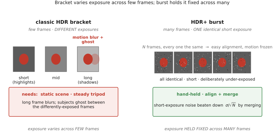
• **see it — recover an underexposed shot, full-frame vs phone**: shoot the *same* underexposed scene as **raw** on a **full-frame** camera and on a **phone**, then **push the exposure up** in software (e.g. +3–4 stops). The full-frame frame cleans up (deep full-well + low read-noise floor → wide dynamic range), while the phone frame breaks down into **shadow noise and banding** as the lift amplifies its read-noise floor — a direct, visible demonstration that **dynamic range scales with photosite / sensor size**, and exactly why phones lean on **burst / HDR+** (Multiple exposure) rather than a single exposure. [fig-underexposure-recovery-ff-vs-phone; photo — paired Fredo full-frame DNG + phone raw] *(also a coding exercise — see [[Exercises & Experiments]])*
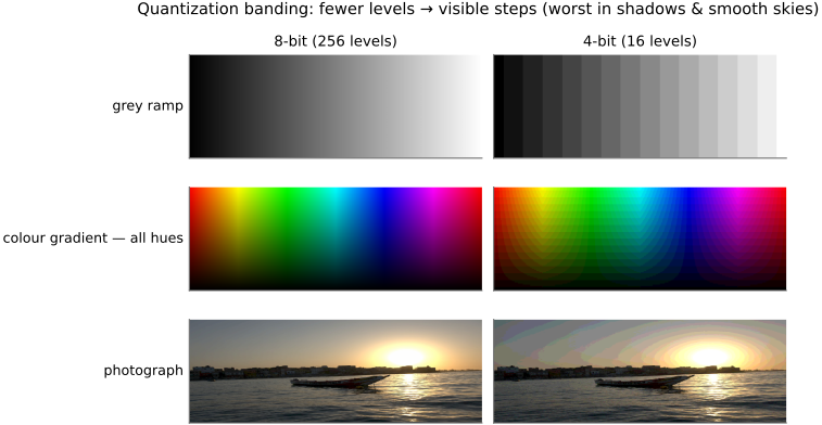
• 💡 **Big lesson (L2.49) — quantization is rarely the real problem**: with enough bits and a sane encoding, it's **noise and dynamic range** (this section) that bite — not the number of levels. The one exception is **gamma / banding in shadows**, which is exactly why gamma encoding exists (allocate codes perceptually); so "rarely" ≠ "never". Reminded again in BASIC → Image representation → *Float vs 8-bit*.
equations
shot noise Poisson (variance = mean), σ ∝ √N, SNR = √N
variances add (shot + read + thermal)
averaging N frames → noise /√N
PSNR = 10·log₁₀(MAX²/MSE)
dynamic range = full-well ÷ read-noise floor
2.13.1 Noise sources
2.13.2 The algebra of noise
2.13.3 Signal-to-noise ratio: it's about ratios
2.13.4 Dynamic range
2.13.5 Regimes, and how close we are to the limits
2.14 Imaging as a linear system
2.15 Imaging as an inverse problem
2.16 Limitations of the medium
2.17 Displays
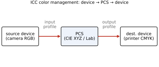
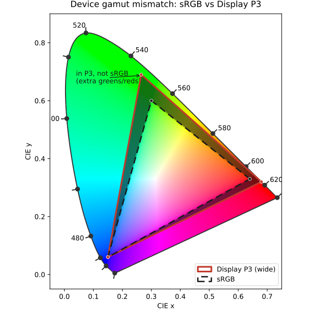
• chapter intro: the last link in the chain. The range of displays (phone, laptop, TV, projector, print) and how their characteristics — size and viewing distance, resolution, dynamic range, gamut, and viewing environment — shape both the experience and the processing. This chapter also carries color management: the ICC workflow and the industry standards that keep color consistent across capture, editing, and display. Forward-reference to [[Integral and immersive imaging]] for near-eye and immersive displays.
Part 3 PHOTOGRAPHY
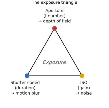
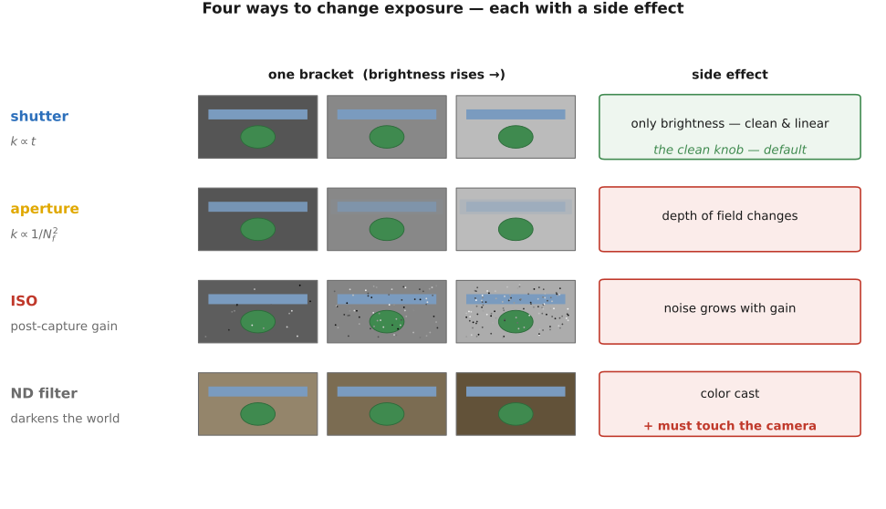
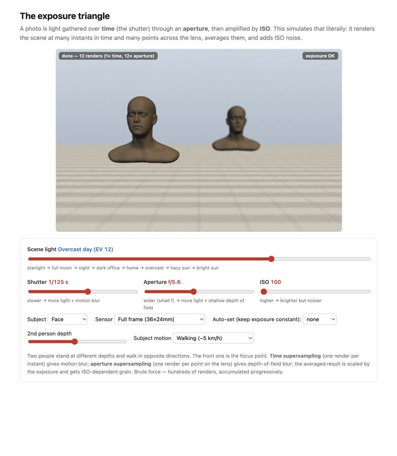
fig-exposure-triangle
fig-exposure-triangle · exposure triangle 🟨
Fundamentals followed light from a source to a perceived color. This part turns to the act of photography itself: how the abstractions of exposure, focus, and focal length become the controls, modes, and hardware of a real camera, and how a phone reaches the same goal by a computational route. It closes by dismantling the myth that the camera is objective. Every "correction," "enhancement," and "restoration" in the rest of the book is a choice with a default, not a neutral truth, and that reframing is the bridge into the computational chapters that follow.
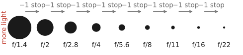
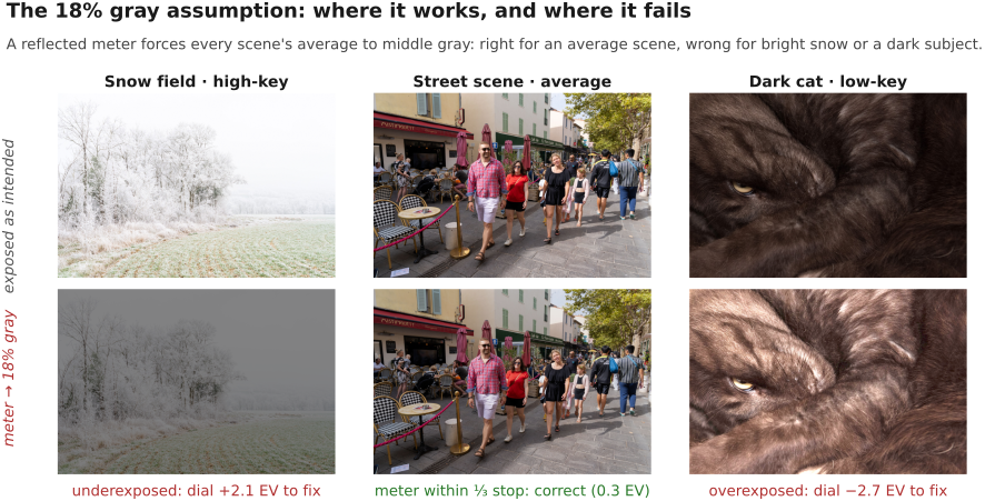
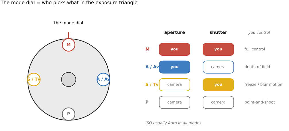
• **Exposure** — shutter, aperture, ISO, stops (Big lesson L3.1), metering and the 18% grey, priority modes, ETTR, and the PASM/auto-ISO mode dial.
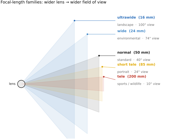
• **Lenses** — focal length and field of view, prime vs zoom, fast vs slow, image stabilization, keeping the glass clean, and filters (polarizer, ND, graduated ND).
• **Focus, autofocus, and depth of field** — CDAF, PDAF, on-sensor dual-pixel, depth-from-defocus, focus modes, and subject/eye detection.
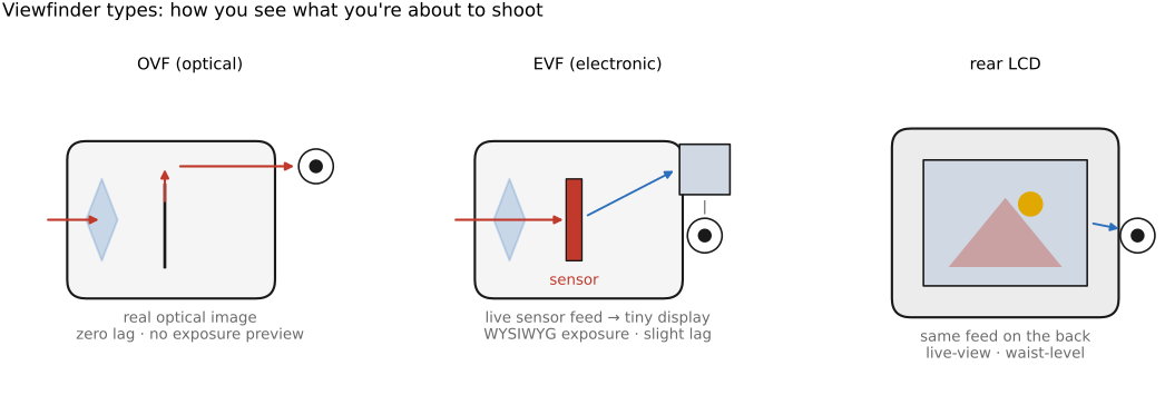
• **Cameras** — the viewfinder, the anatomy of a mirrorless body and of a phone, camera vs phone, the taxonomy of camera types, cameras that measure rather than photograph, and the non-imaging sensor suite.
• **Video** — frame rate and shutter angle, rolling shutter, log profiles, codecs.
• **Illumination and the flash** — goals of lighting; natural illumination (time of day, weather, sky models, golden/blue hour); flash metering (TTL, sync speed and HSS, fill flash); indirect illumination and bounce; multiple-point lighting.
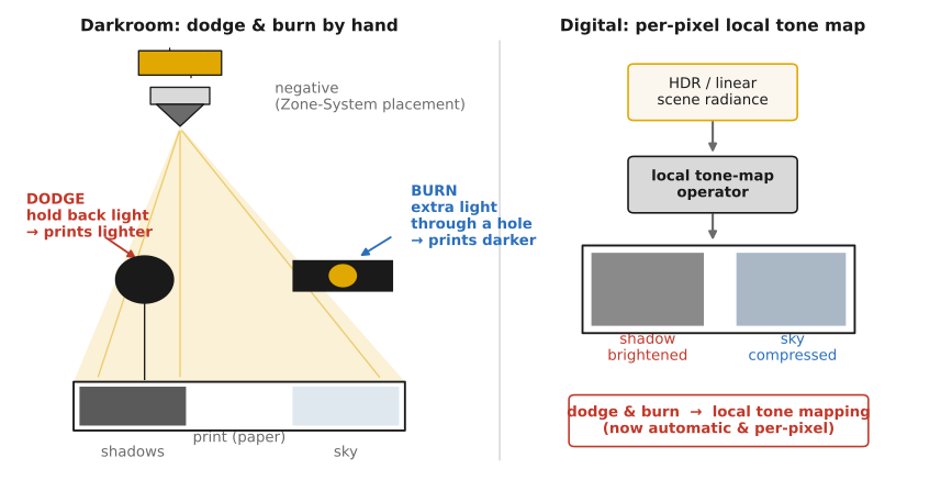
• **Traditional and Digital Darkroom** — the chemical darkroom (develop and print, dodging and burning, the Zone System) and the digital one (parametric raw developers vs pixel editors), every tool an algorithm studied later.
• **Programmability, or the lack thereof** — closed firmware, CHDK/Magic Lantern, the phone camera APIs, and why computation lives on phones.
• **Photographs are usually not passive objective recordings** — the photographer's degrees of freedom, why faithful is not the same as realistic, and the continuum from adjustment to fabrication.
3.1 Exposure
• chapter intro: having built the physics, we now sit behind a real camera — its **controls, modes, and guts** — and see how phones reach the same goal by a wholly different (computational) route
3.2 Lenses
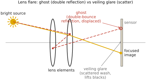
• chapter intro: what a focal length is *for*, fast vs slow, prime vs zoom, image stabilization, keeping the glass clean, and the filters that change the captured light.
3.3 Focus, autofocus, and depth of field
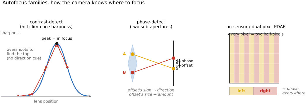
fig-af-families
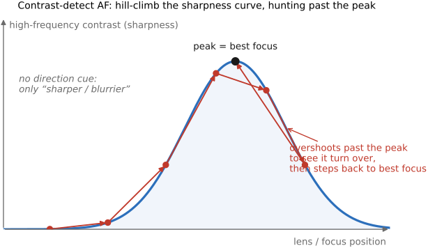
fig-af-families · autofocus families: contrast-detect hill-climb · phase-detect sub-aperture offset · on-sensor/dual-pixel PDAF
fig-telephoto-vs-retrofocus
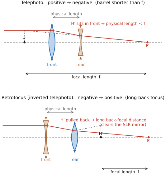
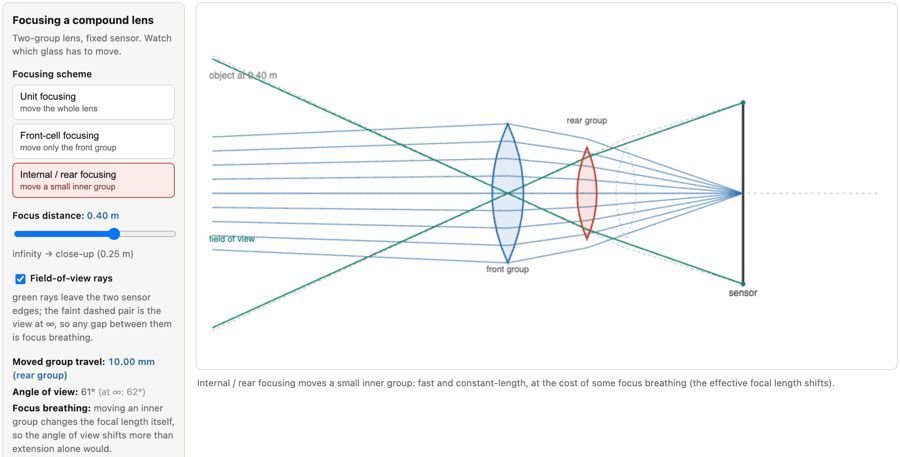
fig-telephoto-vs-retrofocus · two two-group schematics — telephoto (+ then −, principal plane H′ pushed in front → physical length < f) vs retrofocus/inverted-telephoto (− then +, long back-focal distance to clear the SLR mirror); marks f vs physical length, H′, F′
⬜ figure not yet created
phase-detection geometry — in-focus vs too-near vs too-far [fig-pdaf-phase fig-pdaf-phase
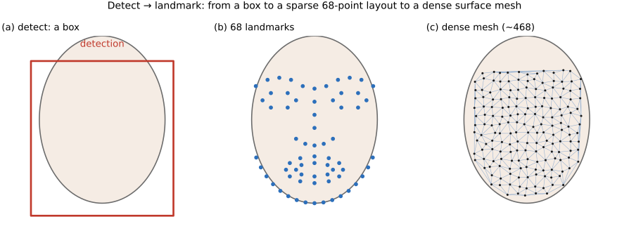
fig-face-landmarks
fig-face-landmarks · face analysis detect→landmark progression: (a) detection box, (b) classic 68-point landmark layout, (c) dense ~468-point surface mesh, over a schematic face (Face tracking, 7.x)
• **the two classic passive AF families**:
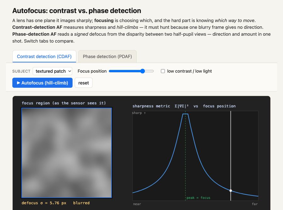
• **contrast-detection (CDAF)**: drive the lens until image **contrast/sharpness is maximal** — accurate but has to **hunt** (it doesn't know which way is "more in focus", only that it overshot); historically slow, common on early mirrorless / compacts
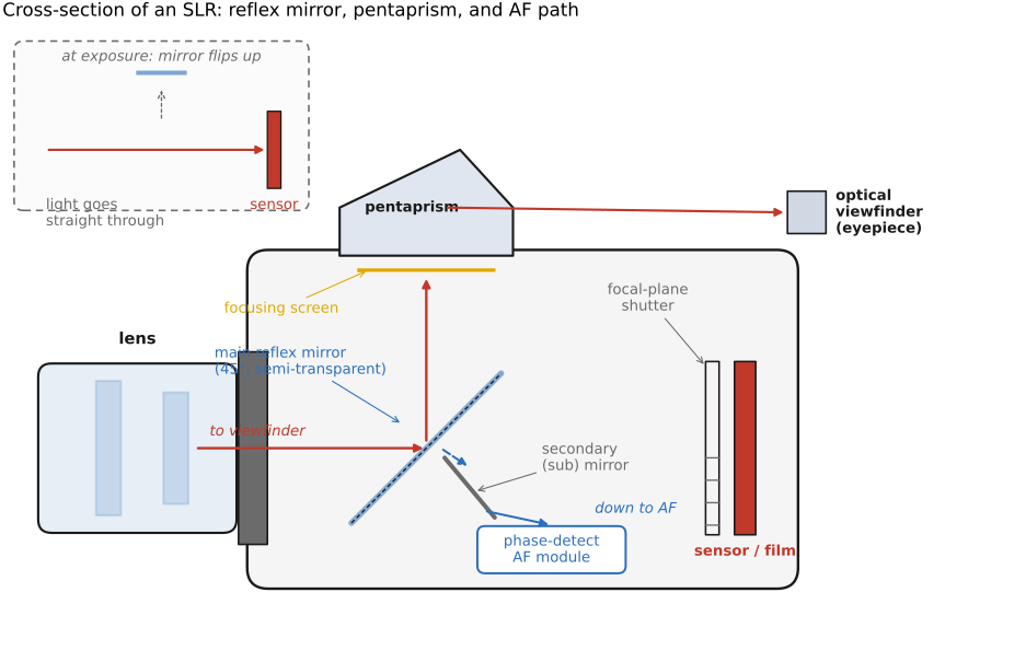
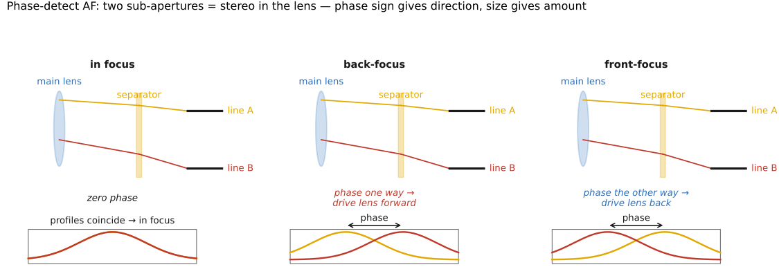
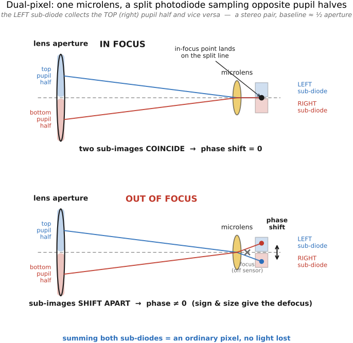
• **phase-detection (PDAF)**: look at the scene through **two opposite edges of the lens** (sub-apertures) → two slightly shifted images; the **phase difference gives the direction *and* amount** of defocus in **one shot**, so the lens moves straight to focus (open-loop, no hunt). Classic SLR mechanism (a dedicated AF sensor under the mirror); it is literally a **tiny stereo measurement**
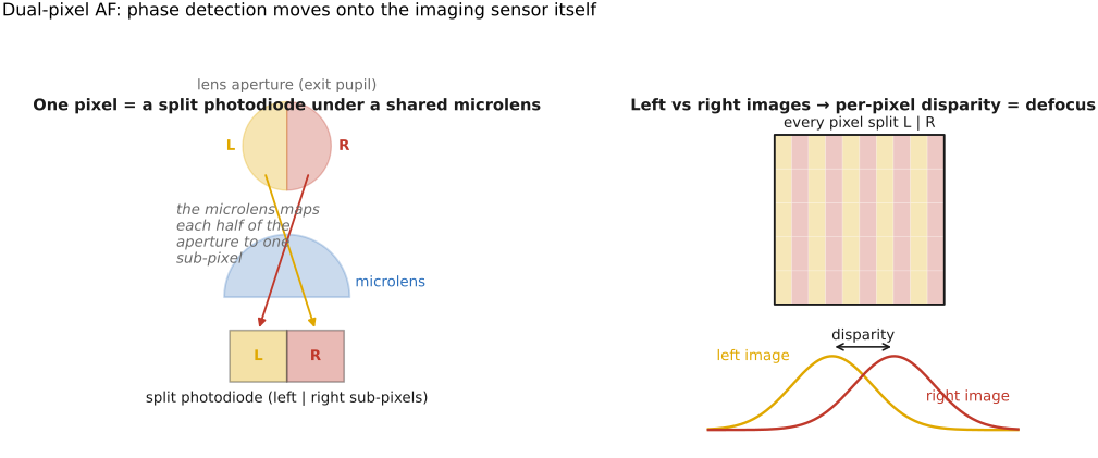
• **on-sensor PDAF / dual-pixel**: mirrorless bodies put phase detection *on the imaging sensor* — masked AF pixels, or **dual-pixel** designs that split each photosite into two halves that see opposite sub-apertures → phase detection at (nearly) every pixel, the best of both worlds (used for Pixel's portrait-mode depth too — a literal micro-stereo pair)
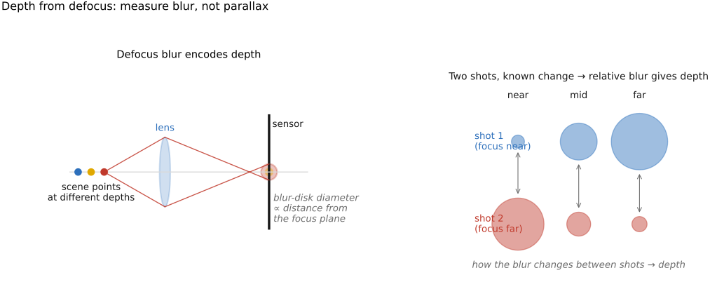
• **depth-from-defocus AF (Panasonic DFD)**: a third route — model how the lens's blur (PSF) changes with focus and read the **defocus direction and amount** from **two frames at slightly different focus**, giving a PDAF-like one-step cue from a plain **contrast** sensor (no phase pixels); rides on CDAF, needs a **per-lens blur profile** (full treatment → Optics, *Focus*)
• **active AF** (for completeness / history): time-of-flight ultrasonic (old Polaroid sonar) and IR rangefinding — work in the dark but limited; distinct from an **AF-assist lamp** that merely adds contrast for passive AF
• **focus modes**: **AF-S / one-shot** (lock once, for still subjects) vs **AF-C / AI-Servo** (track continuously, predict motion, for action); plus **MF** with focus aids (peaking, magnify — see UI)
• **focus selection & automation** — where computation now lives: single-point / zone / wide-area selection, then **subject-detection AF** — **face → eye → animal/bird/vehicle** detect that picks and **tracks** the subject (deep-learning driven; →ML). **Eye-AF** is the headline modern feature for portraits.
• **handling tricks**: **back-button focus** (decouple AF from the shutter button — focus with a thumb button, shutter only releases) and **focus-and-recompose** (lock focus on the subject, then reframe — beware the small focus-plane error at wide apertures / close range)
3.4 Cameras
• chapter intro: the viewfinder and its overlays, the anatomy of a mirrorless body and of a phone, camera vs phone, the taxonomy of camera types, cameras that measure rather than photograph, and the non-imaging sensor suite.
3.4.4 Camera versus phone
3.5 Video
fig-shutter-angle
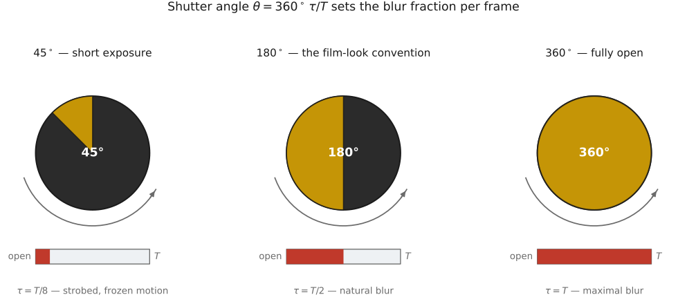
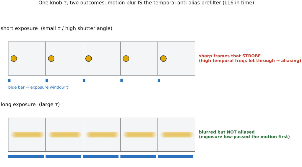
fig-shutter-angle · shutter angle sets the blur — a rotating-disc shutter at $0°/180°/360°$ admitting a smaller/larger fraction of the frame interval $T$; $180°$ ($\tau=T/2$) is the cinematic film-look, small angles strobe 🟨
fig-rolling-shutter-skew
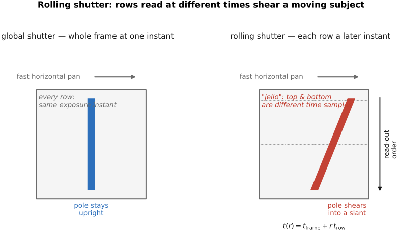
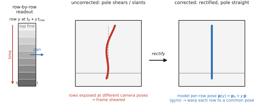
fig-rolling-shutter-skew · rolling-shutter distortion — a global shutter keeping a vertical pole upright under a fast pan vs a rolling shutter where per-row readout $t(r)=t_\text{frame}+r\,t_\text{row}$ shears the pole and smears fan blades (the jello effect) 🟨
• **frame rate & shutter angle**: video sets exposure time as a fraction of the frame interval — the **180° shutter-angle** convention (shutter ≈ ½ the frame time) gives "natural" motion blur; high frame rate → slow motion
• **rolling shutter / "jello"**: CMOS reads the sensor **row by row**, so fast motion (or a fast pan, or a spinning prop) **skews/wobbles** — a **global shutter** avoids it but is rarer/costlier (ties back to CMOS readout in Image measurements as integrals)
• **log / flat profiles + grading**: shoot a **log** (flat, low-contrast) profile to preserve dynamic range, then **color-grade** in post — the video cousin of raw + tone curve
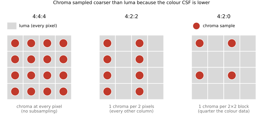
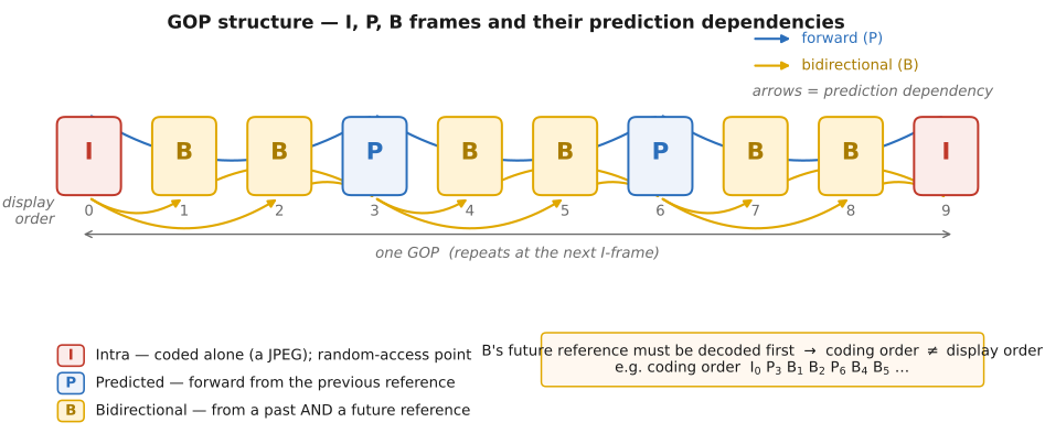
• **codecs & bitrate**: intra- vs inter-frame compression, 8- vs 10-bit, chroma subsampling (4:2:0 vs 4:2:2), bitrate — trade file size vs editing/grading headroom
• *(kept deliberately brief — the algorithms and the full motion treatment are in **Motion/Video**)*
3.6 Illumination and the flash
fig-point-op-levels
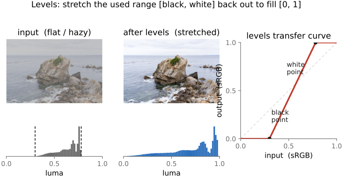
fig-point-op-levels · levels on a real (flat/hazy) photo: bunched-up luma histogram stretched out to fill [0,1] by setting a black point and a white point — input + after + transfer curve with the clip-and-stretch anchors and the two histograms (Point operations → Black point, white point, and levels, BASIC)
fig-wide-angle-perspective-distortion
fig-wide-angle-perspective-distortion · wide-angle perspective distortion: off-axis spheres image as radially-stretched ellipses (flat-sensor geometry), and faces near a wide frame's edge are widened — not a lens flaw; forward-ref to correction (Pinhole image formation)
fig-flash-sync
fig-flash-sync · flash & focal-plane-shutter sync: whole frame ≤ X-sync · slit/partial frame above it · high-speed-sync pulse train; fill-flash noted
fig-telephoto-vs-retrofocus
fig-telephoto-vs-retrofocus · two two-group schematics — telephoto (+ then −, principal plane H′ pushed in front → physical length < f) vs retrofocus/inverted-telephoto (− then +, long back-focal distance to clear the SLR mirror); marks f vs physical length, H′, F′
⬜ figure not yet created
**natural illumination from a physical sky, 3-D interactive [fig-sky-illumination-sim fig-sky-illumination-sim
fig-dof-raydiagram
fig-dof-raydiagram · **interactive** 2-D thin-lens depth-of-field ray diagram + plot: set focal length, f-number, subject distance, circle of confusion and sensor size; the diagram shows the focused cone landing on the sensor and a background point spreading into a blur disk; reads off near/far limits, hyperfocal distance H and magnification; "constant magnification" toggle plots total DoF vs focal length (nearly flat — at fixed framing DoF barely depends on focal length). A lighter companion to the 3-D dof sim.
• **Natural illumination**: sun (hard, small) + sky (soft, huge dome) and their changing ratio; time of day (noon toplight → warm low sun; **golden hour**, **blue hour**); weather (overcast = giant diffuser; haze/aerial perspective); **sky models** (CIE distributions; Perez all-weather, Preetham daylight, Hošek–Wilkie), tuned by turbidity.
• 🖱️ **Interactive (web edition):** a 3-D **natural-illumination / physical-sky simulator** — a head/figure under a modeled sky dome; controls for sun **azimuth/elevation** and **turbidity**; a toggle shows the sky **approximated by many point lights** over the hemisphere (plus a sun key). [fig-sky-illumination-sim; interactive]
• **TTL metering**: the camera fires a **pre-flash**, meters the return **through the lens**, and sets flash power automatically — the flash analog of auto-exposure
• **sync speed & high-speed sync**: a **focal-plane** shutter only fully uncovers the sensor up to its **X-sync speed** (~1/200 s) — faster than that and a moving slit means the flash can't light the whole frame; **high-speed sync (HSS)** pulses the flash rapidly to cover the slit (at a big power cost). A **leaf shutter** (in-lens) opens fully at *any* speed → **syncs at all shutter speeds** (a real advantage for daylight fill).
• **fill flash**: in harsh/backlit light, add flash at **−1 to −2 EV** (the slides say −1.5 to −2, i.e. 3–4× below ambient) to **open the shadows** without looking flashed — it's **dynamic-range management**, not "more light"
• **bounce & off-camera**: never bare flash head-on (flat, harsh, red-eye) — **bounce** off a ceiling/wall (~45°) or use a diffuser to enlarge the source → softer light; **off-camera** flash gives directional, shaped light (→ Computational illumination; computational bounce flash, Davis SIGA 2016)
• 🖱️ **Interactive (web edition):** a live **portrait-lighting simulator** — three soft area lights (key / fill / kicker, each with azimuth, elevation, size/softness, intensity, and colour) on a 3D face, with **area-light-supersampled soft shadows** and a physiological melanin/hemoglobin skin model; a from-behind "setup" view shows the lights as studio umbrellas plus the camera, and lighting presets (butterfly, loop, Rembrandt, split, clamshell, rim) let you feel how light *placement and size* sculpt a face. [fig-portrait-lighting-sim; interactive] *(3D studio umbrella generated with Meshy AI — acknowledge in the caption)*
3.7 Traditional and Digital Darkroom
3.8 Programmability, or the lack thereof
fig-bokeh-shapes
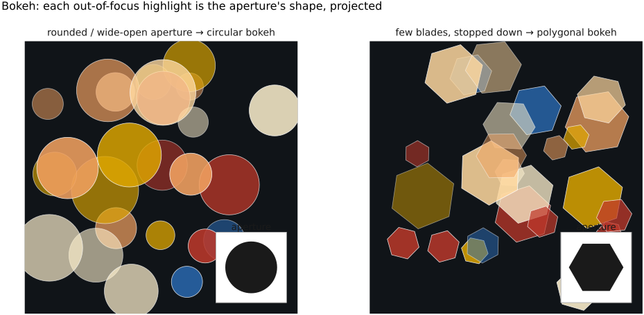
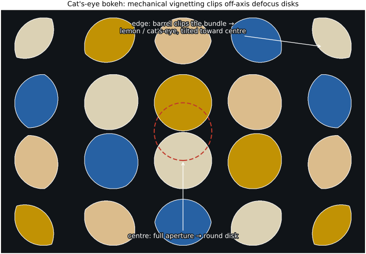
fig-bokeh-shapes · bokeh: out-of-focus highlights take the aperture's shape — circular (many blades / wide open) vs polygonal (few blades, stopped down); synthetic defocus-disk fields + aperture insets
• most cameras run **closed firmware**: you cannot run your own code on them, so the **computational-photography ideas in this book can't be tried on a stock camera** — a real obstacle for experimentation
• the **hacks**: **CHDK** (Canon PowerShot) and **Magic Lantern** (Canon DSLRs) are community firmware add-ons that expose scripting, raw video, bracketing, intervalometers, and focus stacking — born exactly because the manufacturers wouldn't
• the **open road**: **Android's Camera2 / CameraX** API (and Google's earlier FCam research camera) expose per-frame control of exposure / focus / gain and access to **raw burst** — which is *why phones, not cameras, became the home of computational photography*
• the **maker road**: a **Raspberry Pi + camera module** (the HQ camera, driven by **libcamera / picamera2**) is a cheap, fully **open and programmable** camera — per-frame exposure/gain control and **raw** access on a hobbyist board — the natural platform for *trying this book's algorithms* and building DIY computational cameras
• **why this matters for the book**: our algorithms (HDR+, burst denoising, computational bokeh) need **programmable capture** — control of the per-frame integral and access to raw; the platform that grants it is where the research happens
3.9 Photographs are usually not passive objective recordings
Part 4 BASIC IMAGE PROCESSING AND ISP
At the end of this part, the readers will be able to implement a complete ISP or very basic version of a photo editing software (mini lightroom) with exposure, contrast, etc.
4.1 Image representation
fig-image-memory-layout
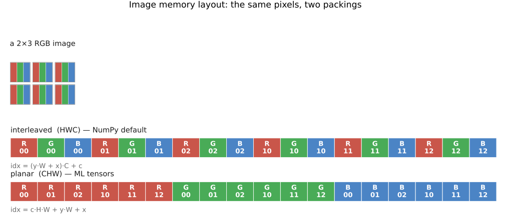
fig-image-memory-layout · a 2×3 RGB image packed into 1-D memory two ways — interleaved HWC (NumPy) vs planar CHW (ML), with the stride formulas (Image representation, BASIC) 🟨
fig-edge-handling-photo
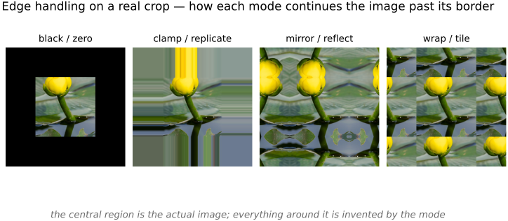
fig-edge-handling-photo · the four edge modes on a real crop — black / clamp / mirror / wrap continued past the border; real-image companion to `fig-edge-handling` (Image representation → falling off the edge, BASIC)
4.2 What the numbers mean
4.3 Developing, Testing and Debugging
4.4 Point operations
fig-operation-types
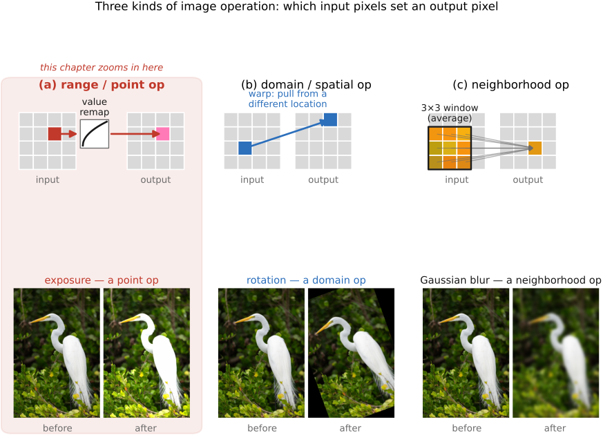
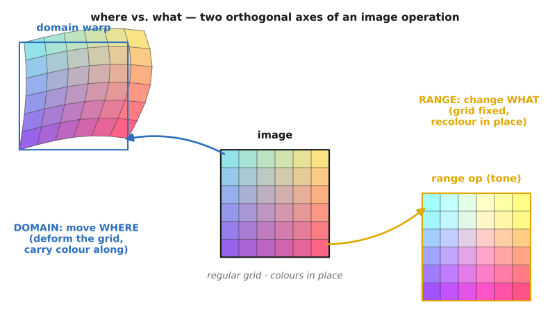
fig-operation-types · the three image-operation types — range (point) vs domain (spatial) vs neighborhood (Values / point ops, BASIC) 🟨
4.4.9 Converting to black and white
4.5 Histograms
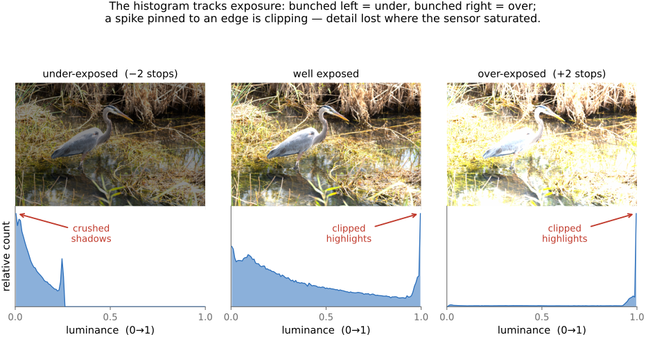
fig-histogram
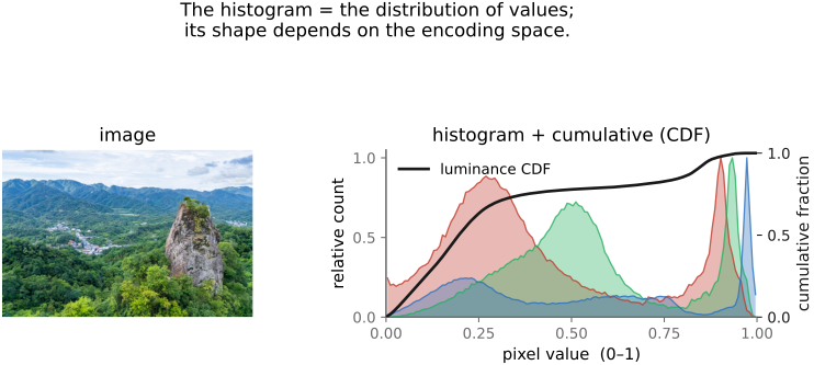
fig-histogram · an image histogram (per-channel) + cumulative histogram; its shape depends on the encoding space (BASIC tone mapping) 🟨
fig-histogram-encoding-spaces
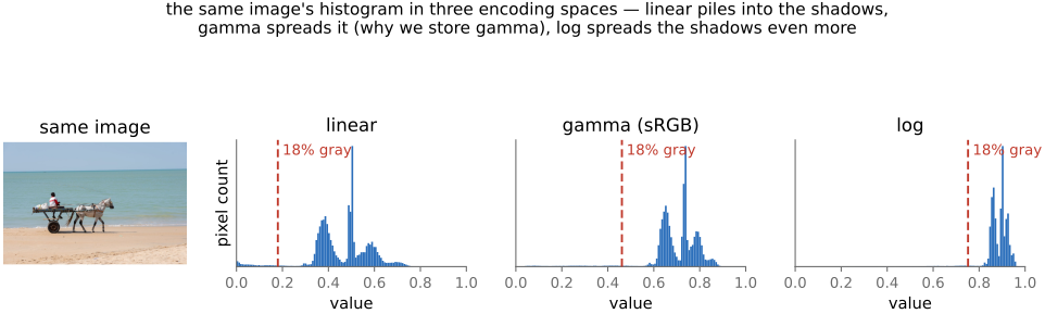
fig-histogram-encoding-spaces · the same image's luminance histogram in linear / gamma (sRGB) / log; 18% gray marked at 0.18 / ~0.46 / ~0.75 — the encoding reshapes the value axis (BASIC histograms) 🟩
fig-histogram-equalization
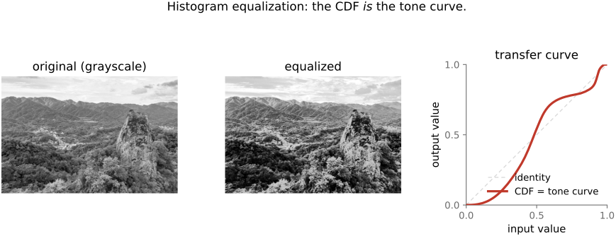
fig-histogram-equalization · histogram equalization — the CDF used as the transfer curve, before/after (BASIC) 🟨
fig-histogram-matching
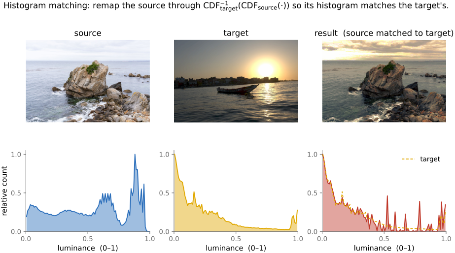
fig-histogram-matching · histogram matching — source + target images and their histograms → matched result, with the composed transfer curve $\text{CDF}_\text{tgt}^{-1}\circ\text{CDF}_\text{src}$ (BASIC histograms)
• the **histogram** — the distribution of pixel values — is the natural companion to point operations: this short chapter is how to *read* it, and how it can *drive* an automatic tone curve
4.6 Global tone mapping
fig-reinhard-curve
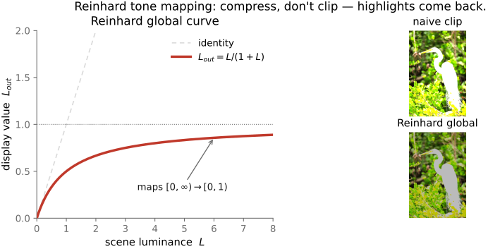
fig-reinhard-curve · the Reinhard global tone curve L/(1+L) mapping [0,∞)→[0,1); naive clip vs Reinhard on a simulated-HDR image (BASIC) 🟨
fig-tonemap-real
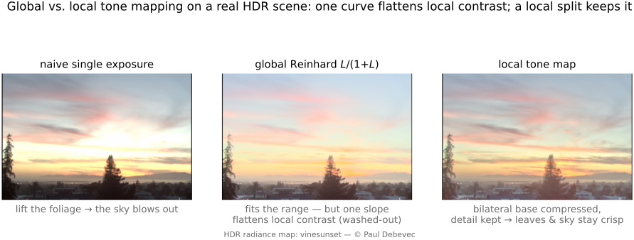
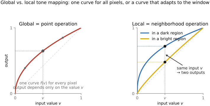
fig-tonemap-real · global vs local tone mapping RESULT on a real HDR photo (seal at marina): naive single exposure · global Reinhard (one slope flattens local contrast → hazy) · local bilateral base+detail split (range fits, detail stays crisp) — real-image companion to `fig-tonemap-global-vs-local` (BASIC tone mapping)
fig-zone-system
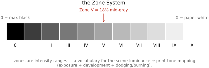
fig-zone-system · the Zone System strip 0–X, Zone V = 18% mid-grey (scene → print) (BASIC) 🟨
• a **quick intro** here (full treatment in the HDR chapter): tone mapping = choosing the **mapping from scene tones to display tones**, the natural payoff of point operations
4.6.8 HDR on every screen: the gain map
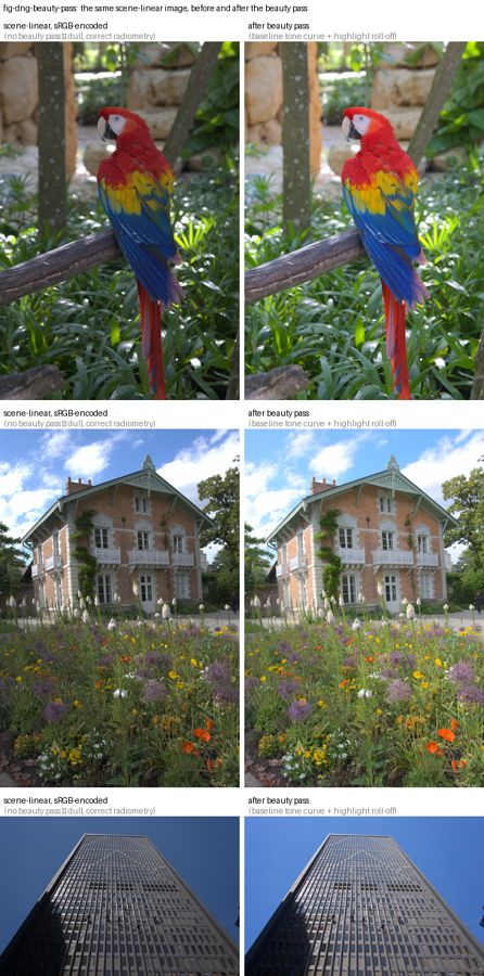
4.7 Beauty curves: the camera "look"
4.8 Neighborhood operations and convolution
fig-convolution-slide
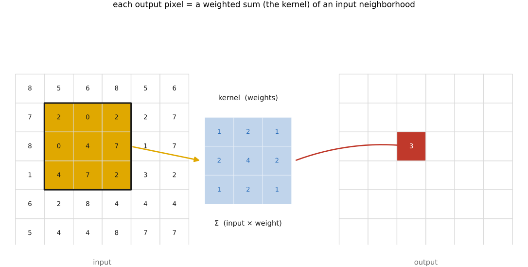
fig-convolution-slide · a kernel sliding over an image, weighted-summing a neighborhood into one output pixel (Convolution, BASIC) 🟨
fig-convolution-flip
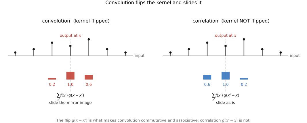
fig-convolution-flip · the flip: where-from vs where-to — convolution `g(x−x')` vs correlation 🟨
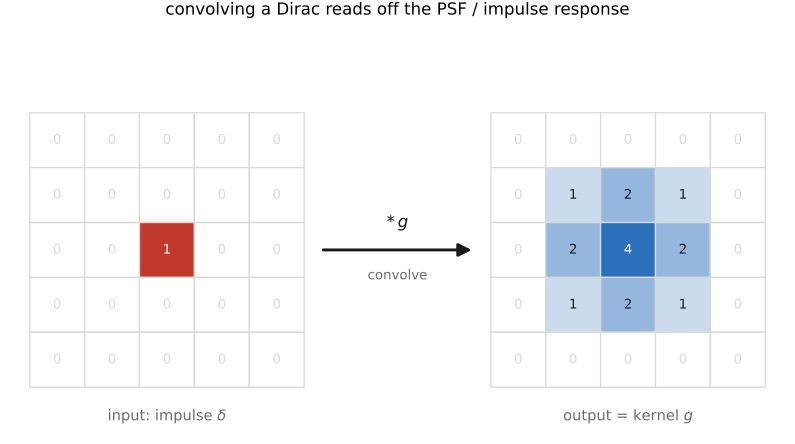
fig-psf-impulse
fig-psf-impulse · impulse in → kernel out: convolving a Dirac reads off the PSF / impulse response 🟨
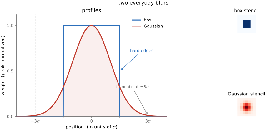
fig-blur-zoo
fig-blur-zoo · box vs Gaussian kernels — profiles + 2-D stencils, Gaussian truncated at ~3σ 🟨
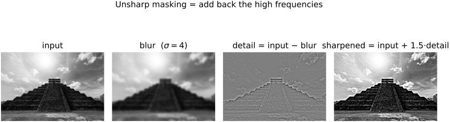
fig-unsharp-mask
fig-unsharp-mask · unsharp-mask decomposition: input − blur = detail (high-pass), output = input + k·detail 🟨
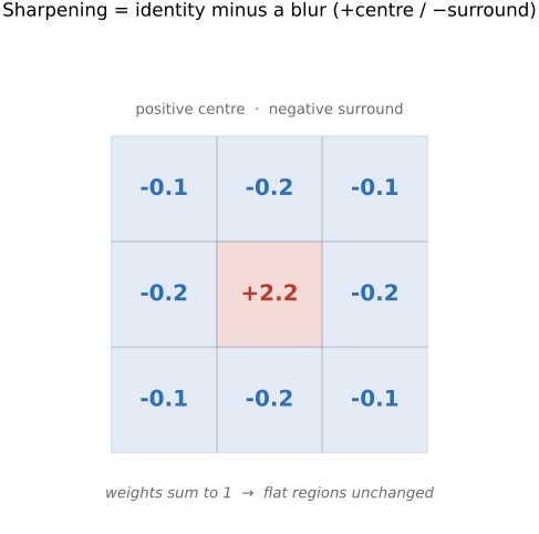
fig-sharpen-kernel
fig-sharpen-kernel · the sharpening kernel δ − blur as a +centre / −surround stencil 🟨
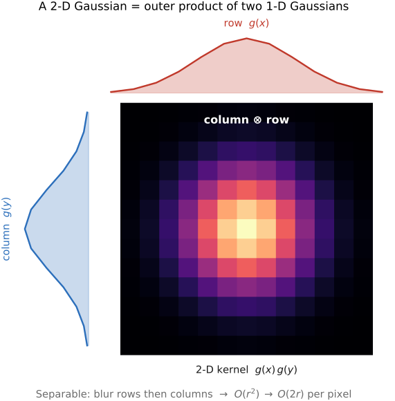
fig-separable
fig-separable · separability — a 2-D Gaussian = 1-D ⊗ 1-D (blur rows then columns); O(r²) → O(2r) 🟨
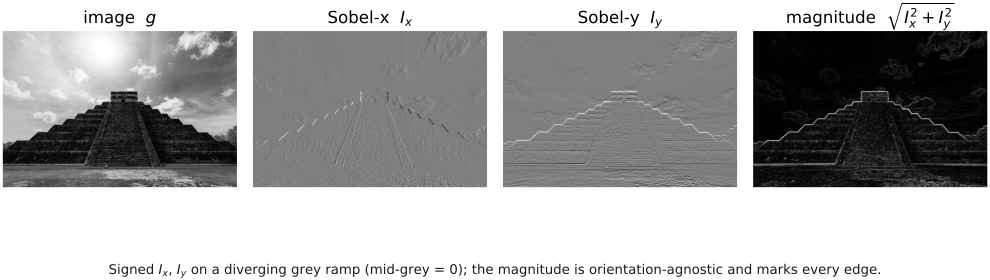
fig-gradient-sobel
fig-gradient-sobel · Sobel x / y → gradient magnitude (edge strength) on an image 🟨
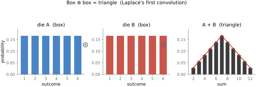
fig-convolution-probability
fig-convolution-probability · convolution as the sum of random variables: box ⊛ box = triangle (two dice) 🟨
equations
convolution (I*g)(x) = Σ I(x')·g(x−x')
Gaussian g(x) ∝ exp(−x²/2σ²)
unsharp out = in + k·(in − blur(in))
sharpening kernel δ − g
4.8.9 Is imaging blur usually a shift-invariant convolution?
4.9 Sharpening
fig-unsharp-mask
fig-unsharp-mask · unsharp-mask decomposition: input − blur = detail (high-pass), output = input + k·detail 🟨
fig-sharpen-kernel
fig-sharpen-kernel · the sharpening kernel δ − blur as a +centre / −surround stencil 🟨
4.10 Fourier
fig-fourier-basis-matrix
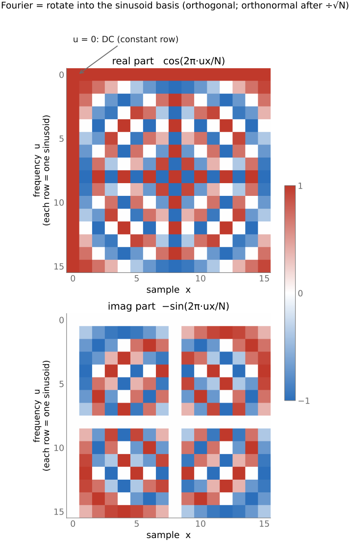
fig-fourier-basis-matrix · the DFT as a change-of-basis matrix (real & imaginary parts) 🟨
fig-sine-eigenvectors
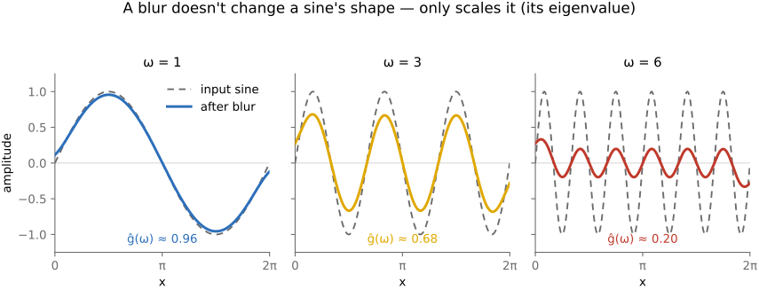
fig-sine-eigenvectors · sine waves are the eigenvectors of convolution: same wave out, only amplitude/phase change 🟨
fig-motion-blur-calculator
fig-motion-blur-calculator · live motion-blur calculator: a 3-D scene (walking figure or a car) imaged by a virtual camera, the blur rendered by **temporal supersampling** (many instants across the exposure, averaged). Set resolution / sensor / focal length (35 mm-equiv) / distance / exposure, add camera-shake **rates** in rotation (pitch/yaw/roll) and translation (x/y/z) plus a subject speed; the readout gives the blur at the subject in world (cm/m/in) and screen (px / % width) units, broken down by source. A per-pixel **G-buffer** (depth + subject mask) drives exact motion-vector arrows and a blur-magnitude heatmap: the subject carries its own motion, the background only camera shake. Environment backdrops + car colour picker. Static fallback is a screenshot. *3D models generated with Meshy AI.*
fig-fourier-magnitude-phase
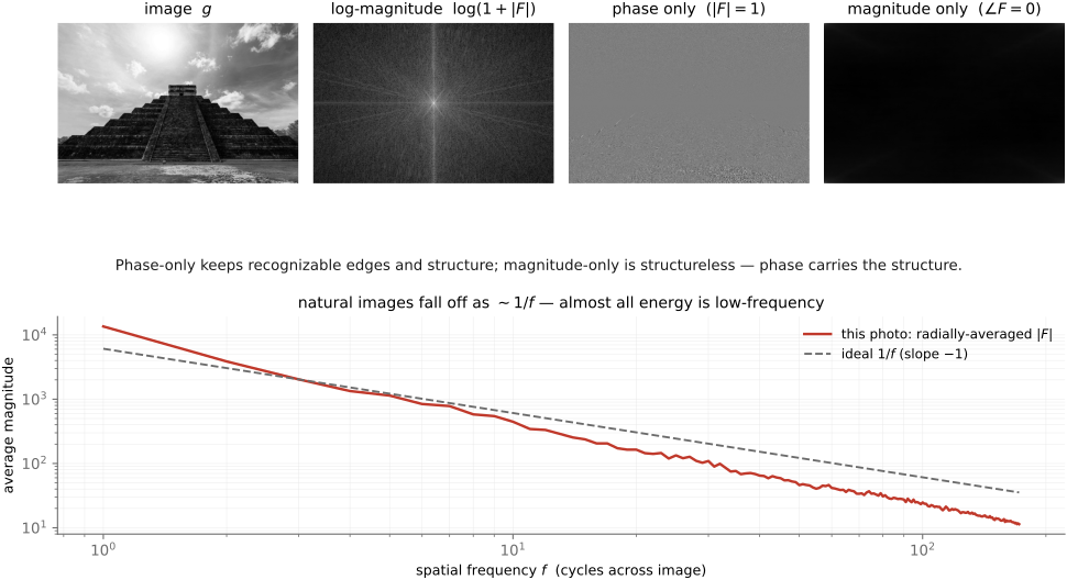
fig-fourier-magnitude-phase · an image's Fourier magnitude & phase, and the phase-swap demo (phase carries structure) 🟨
fig-compact-space-frequency
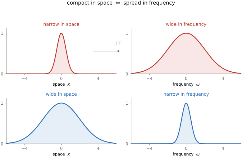
fig-compact-space-frequency · compact in space ⇔ spread in frequency (narrow vs wide Gaussian and its transform) 🟨
fig-aliasing
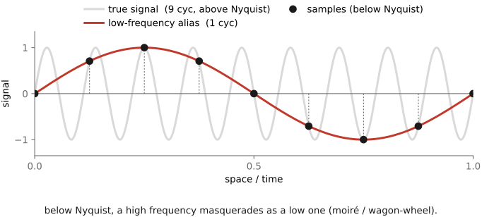
fig-aliasing · sampling a sine too coarsely → aliasing (high frequency folds to a low one) 🟨
fig-sampling-comb
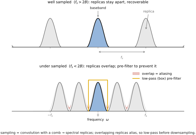
fig-sampling-comb · sampling = multiply by a comb → spectral replicas; pre-filter (low-pass) before downsampling 🟨
fig-sinc-vs-practical
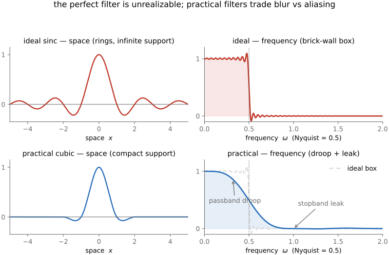
fig-sinc-vs-practical · ideal sinc reconstruction vs a practical filter, in space and frequency 🟨
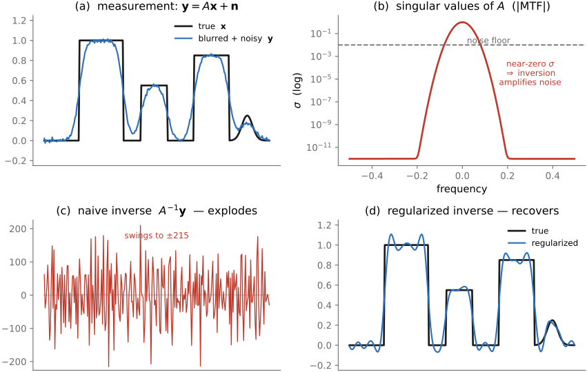
fig-deblur-preview
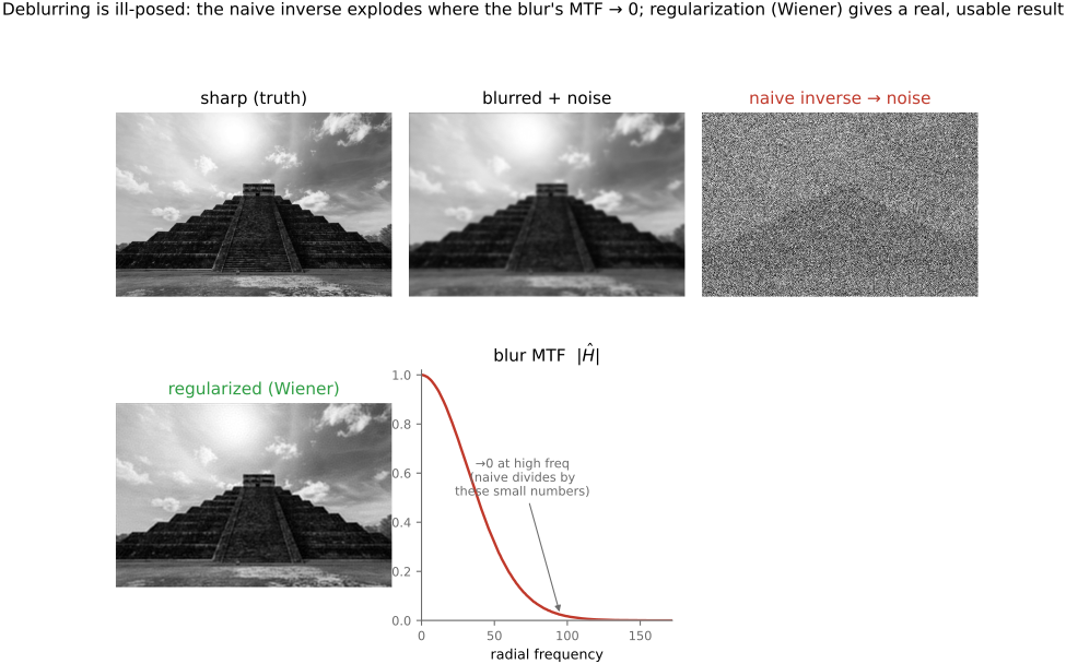
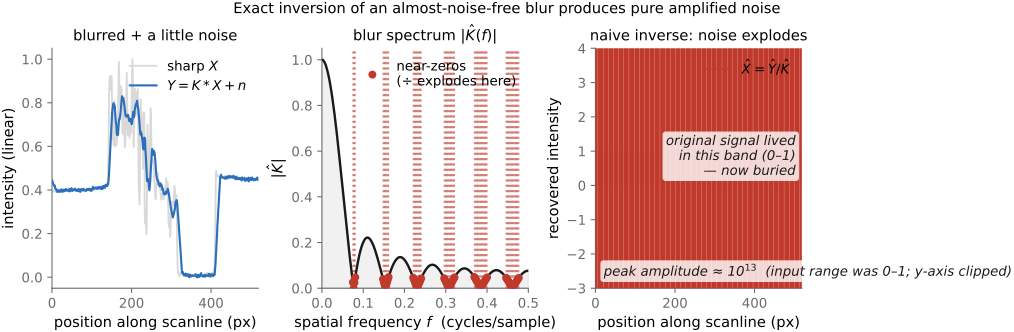
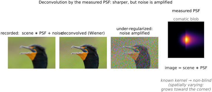
fig-deblur-preview · the deblur preview: sharp → blurred + noise → naive inverse amplifies noise; MTF 🟨
fig-diagonalize-2x2
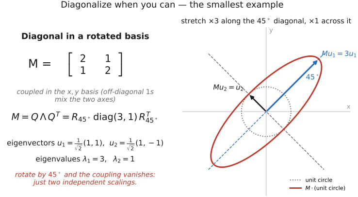
fig-diagonalize-2x2 ·
fig-fourier-conventions
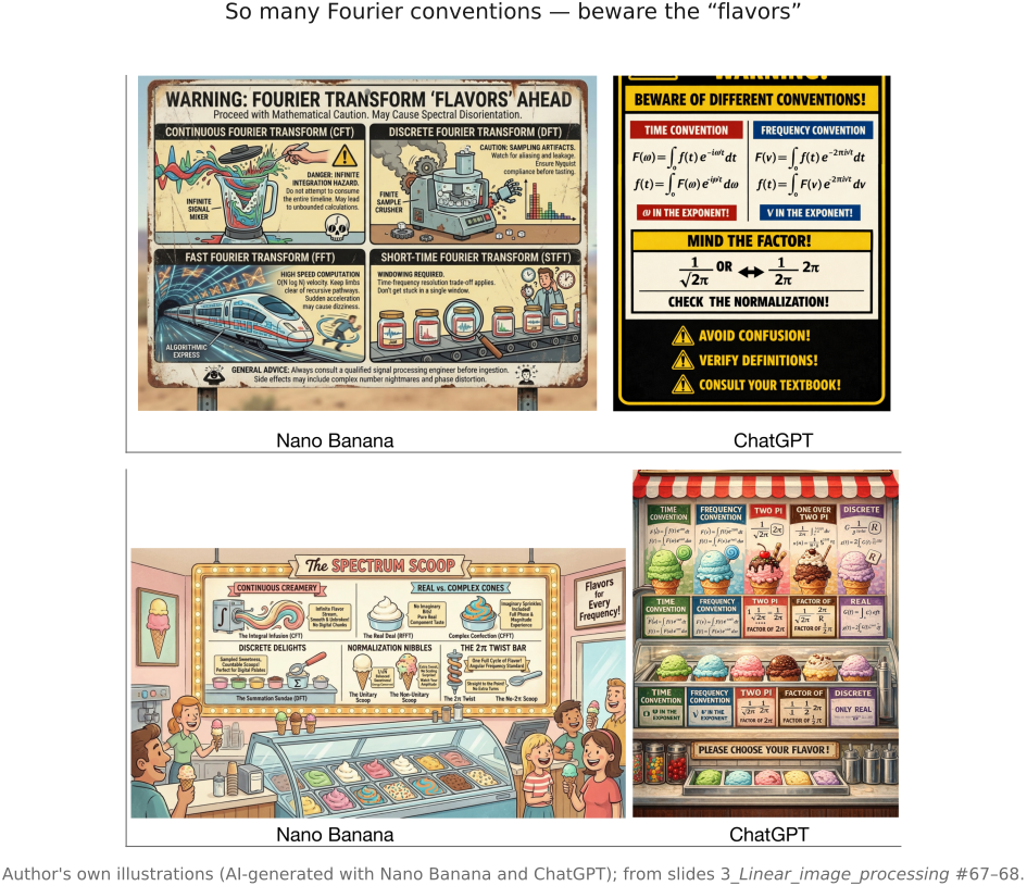
fig-fourier-conventions ·
fig-heat-diffusion-1d
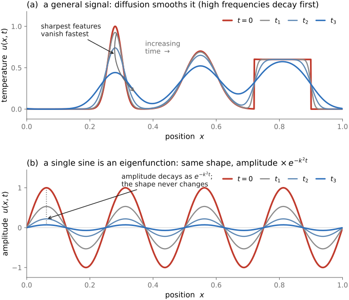
fig-heat-diffusion-1d ·
equations
DFT Î(u) = Σ I(x)·e^{−2πi ux/N}
Euler e^{iθ} = cos θ + i sin θ
convolution theorem ℱ{I*g} = ηĝ
eigen-relation g * e^{iωx} = ĝ(ω)·e^{iωx}
Nyquist — sample > 2× the highest frequency
4.10.7 A small bestiary of transforms
4.11 Sampling, downsampling, and aliasing
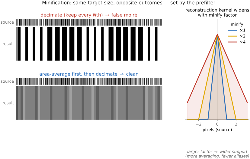
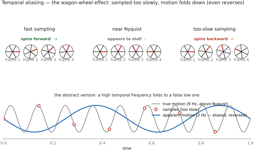
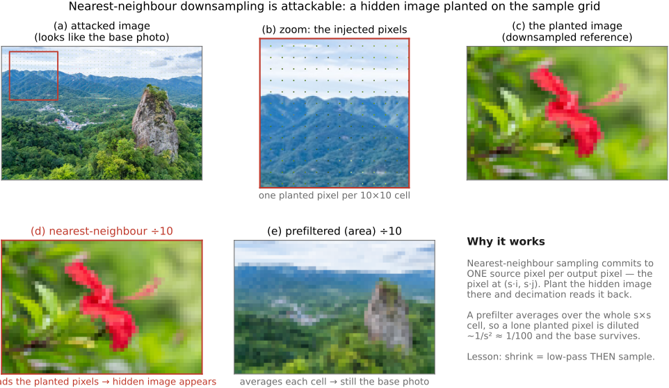
• promoted from a section of [[#Fourier]] into its own chapter (it earns one): a digital image is a **sampling** of a continuous scene, and detail finer than the grid **aliases** — folds down to a wrong, low frequency (moiré, wagon-wheel).
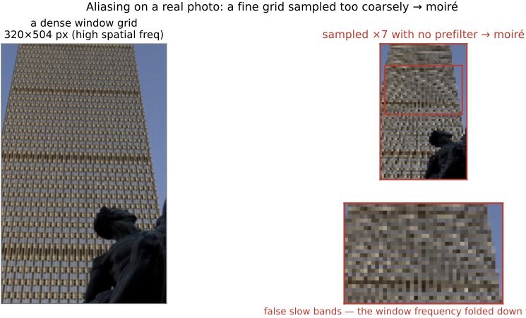
• **aliasing = a high frequency in disguise** (sine sampled below 2×/cycle → looks like a slower sine); 2-D version = moiré on a facade. Figures: `fig-aliasing`, `fig-aliasing-photo`.
• **Nyquist–Shannon**: sample at >2× the highest frequency; the **Nyquist frequency** is half the sampling rate; above it folds down irreversibly.
• **frequency-domain mechanism**: sampling is **multiplication by a Dirac comb** in space, so by the convolution theorem it becomes a **convolution in Fourier** — but by an unusually *simple* spectrum. The comb is **self-dual**: the Fourier transform of a Dirac comb is **another train of Diracs** (spaced at the sampling rate). And that is exactly why sampling is *easy* to reason about in Fourier: convolving by a single Dirac is just a **shift**, so convolving by a *train* of Diracs is just a **sum of shifted copies**. The spectrum is simply **replicated** at every multiple of the sampling rate — no smearing, just shifts. (This is the payoff of Fourier being built on the **shift theorem**: the one convolution that would otherwise be messy collapses into pure translation.) Band-limited copies sit apart; too-wide copies **overlap** = aliasing (`fig-sampling-comb`). Big lesson **L4.13**.
• **cure**: low-pass **pre-filter** (blur) *before* downsampling. Interactive demos: `fig-sampling-1d-demo` (1-D sampling/aliasing/pre-filter, tick-marked samples + spectrum) and `fig-sampling-2d-demo` (downsample the Prudential facade with/without pre-filter → moiré on/off).
• sidebars: aliasing **without** Fourier (pixel = area average); aliasing **on purpose** (KinéCam moiré encodes camera motion).
• **ideal sinc** reconstruction (perfect frequency box ⇒ infinite spatial ripple) is unreachable; practical filters compromise (`fig-sinc-vs-practical`) — handed off to [[#Resampling and upsampling]].
• xref: built on [[#Fourier]]; reconstruction / upsampling lives in [[#Resampling and upsampling]].
4.11.1 Aliasing: a high frequency in disguise
4.11.2 Nyquist and the sampling theorem
4.11.3 In two dimensions, aliasing has a direction
4.11.4 Sampling in the frequency domain: spectral replicas
4.11.5 Seeing it: sampling and pre-filtering, hands on
4.11.6 The ideal reconstruction filter: sinc, and why it is unreachable
4.12 Resampling and upsampling
fig-resample-forward-inverse
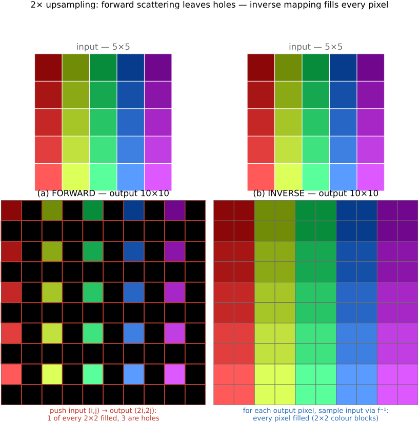
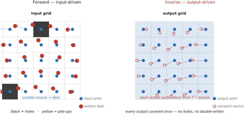
fig-resample-forward-inverse · concrete 2× upsampling on a 5×5 → 10×10 rainbow grid: FORWARD pushes input (i,j)→output (2i,2j) so 1 of every 2×2 output block is filled and 3 are black holes (regular lattice of gaps); INVERSE loops output, samples input via f⁻¹ (nearest) → every pixel filled (2×2 colour blocks). Forward leaves holes, inverse fills everything (Resampling, BASIC)
fig-linear-interp-1d
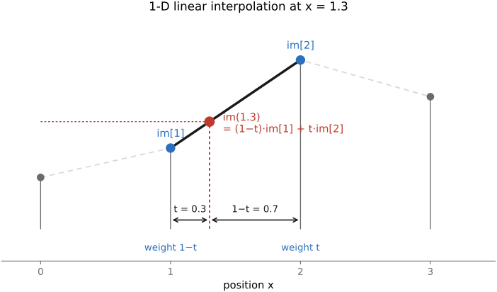
fig-linear-interp-1d · 1-D linear interpolation — `im[1.3]` from its two neighbours 🟨
fig-bilinear
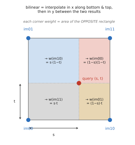
fig-bilinear · bilinear interpolation — the 4-neighbour weighting on the unit square 🟨
fig-resample-kernels-real
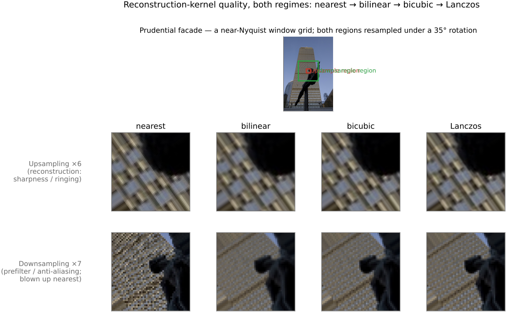
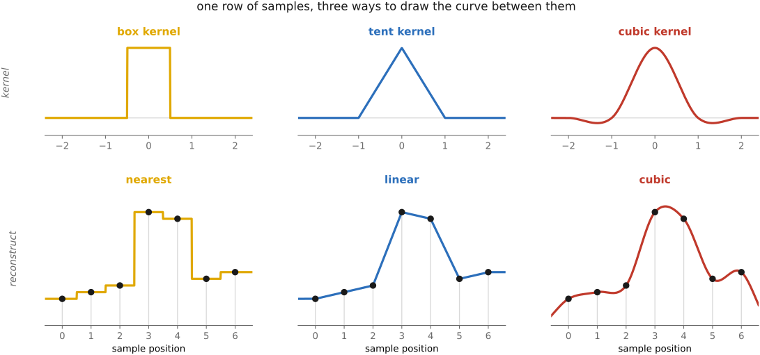
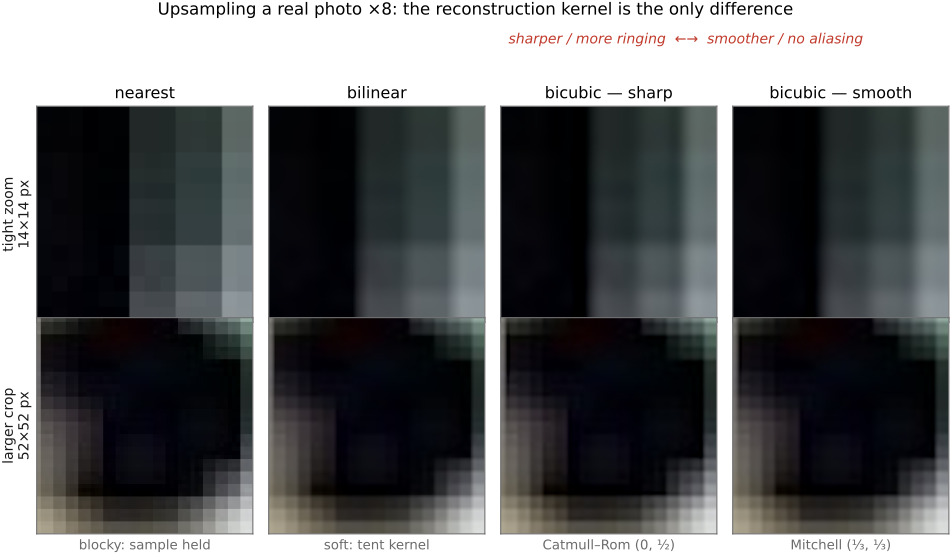
fig-resample-kernels-real · the kernel ladder on a REAL photo (Boston skyline + rainbow) resampled under a 35° rotation, magnified on a detail: nearest (blocky) → bilinear (smeared) → bicubic (edges restored) → Lanczos (sharpest) — adds Lanczos + the rotation case to `fig-interp-comparison`
fig-reconstruction-pipeline
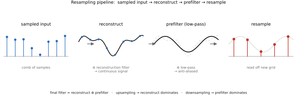
fig-reconstruction-pipeline · the resampling pipeline: sample → reconstruct → prefilter → resample 🟨
fig-aliasing-photo
fig-aliasing-photo · aliasing/moiré on a real photo: a window-grid facade decimated with no prefilter folds into moiré bands — the 2-D, real-image companion to `fig-aliasing` (Sampling and aliasing)
equations
1-D linear interp
general resample out(x) = Σ I(x')·k(f⁻¹(x) − x')
Lanczos `sinc(πx)·sinc(πx/a)`
Mitchell–Netravali cubic (B, C)
4.13 Pyramids and wavelets
fig-gaussian-pyramid
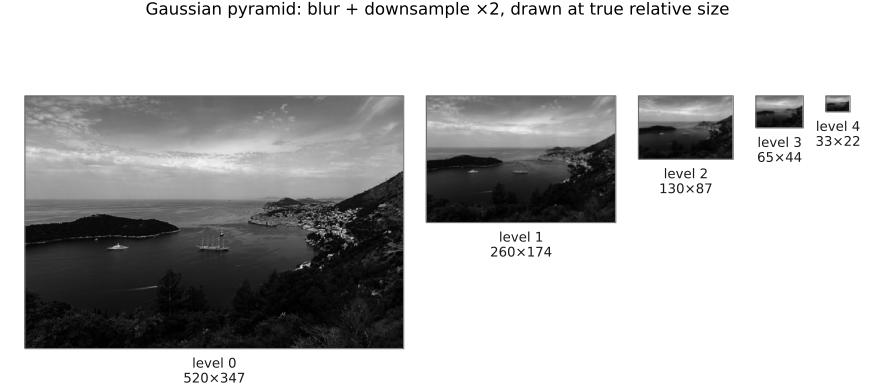
fig-gaussian-pyramid · the Gaussian pyramid — repeated blur + downsample tower (Pyramids, BASIC) 🟨
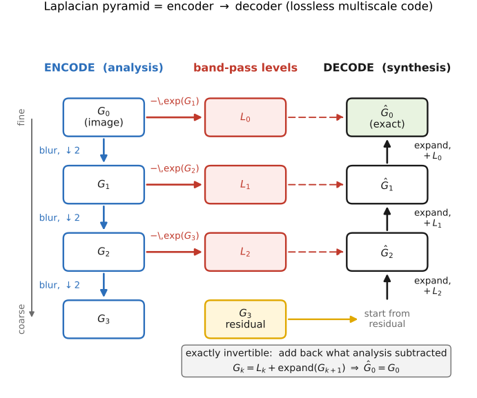
fig-laplacian-pyramid
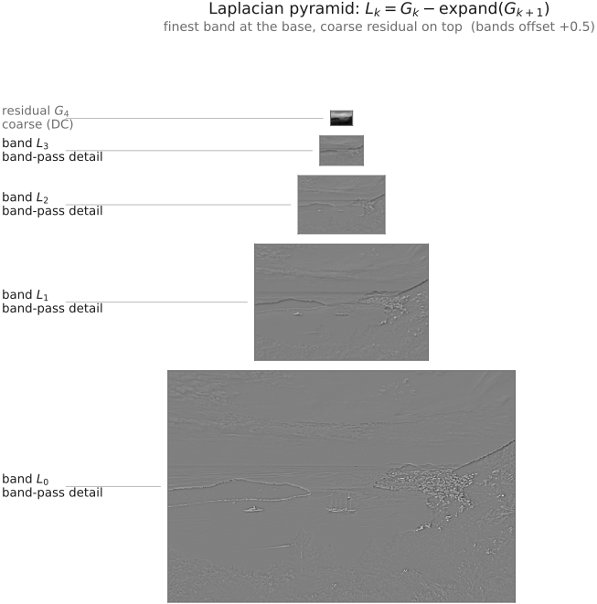
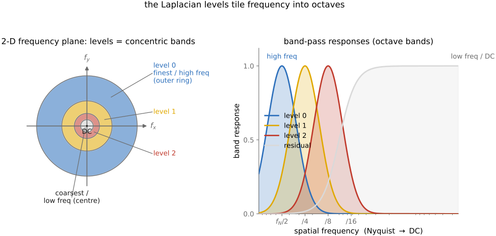
fig-laplacian-pyramid · the Laplacian pyramid — band-pass levels (G_k − expand(G_{k+1})) 🟨
fig-pyramid-encode-decode
fig-pyramid-encode-decode · the Laplacian pyramid as an encoder → decoder (exact reconstruction) 🟨
fig-pyramid-frequency-bands
fig-pyramid-frequency-bands · each pyramid level = a frequency band (concentric Fourier rings) 🟨
fig-kernel-spectra
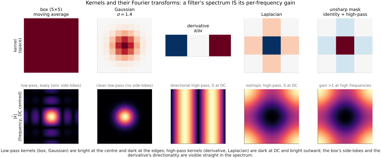
fig-kernel-spectra · five common kernels (box, Gaussian, derivative ∂/∂x, Laplacian, unsharp mask) shown in space and as their Fourier magnitudes — a filter's spectrum IS its per-frequency gain (low-pass leaky vs clean, directional/isotropic high-pass, boosting)
fig-coring
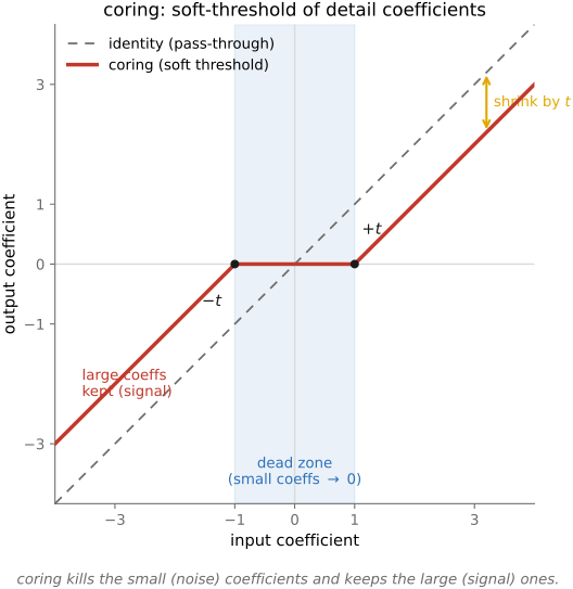
fig-coring · coring — zero the small detail coefficients (noise), keep the large ones 🟨
equations
reduce / expand (blur + ↓2 / ↑2 + blur)
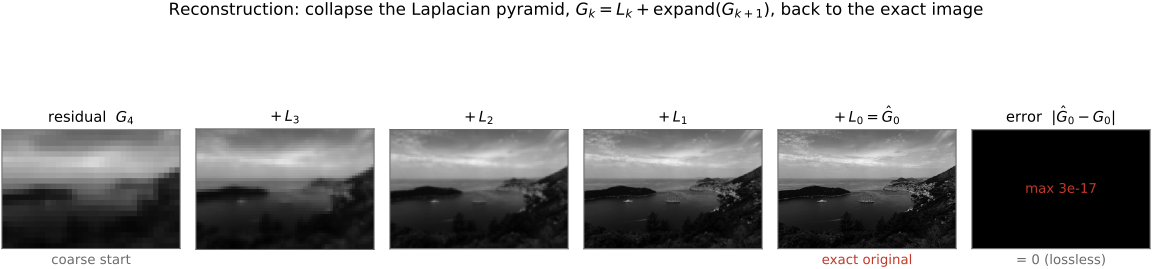
L_k = G_k − expand(G_{k+1})
reconstruction G_k = L_k + expand(G_{k+1})
4.13.10 Pyramid blending
4.13.11 Other applications
4.14 Image metrics
fig-ssim-vs-mse
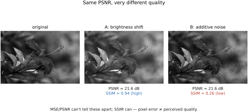
fig-ssim-vs-mse · same PSNR, very different SSIM — pixel error ≠ perceived quality (Image metrics, BASIC) 🟨
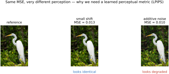
• we **often need to compare two images** — fidelity, alignment, an ML training loss
equations
MSE = mean(‖I−J‖²)
PSNR = 10·log₁₀(MAX²/MSE)
SSIM = luminance·contrast·structure (local windows)
4.15 Denoising basics
fig-denoising-before-after
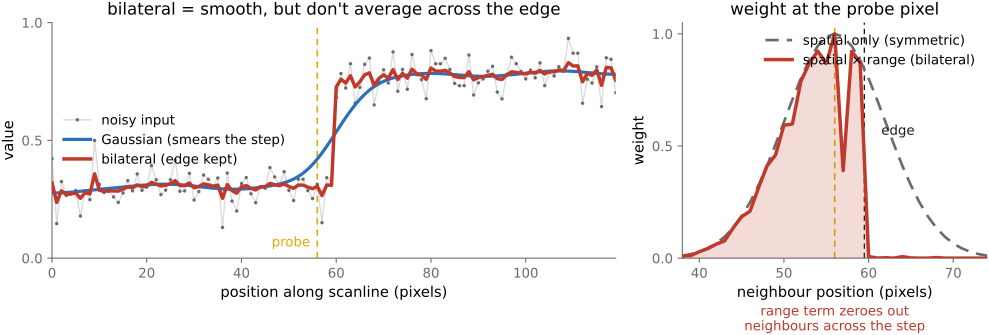
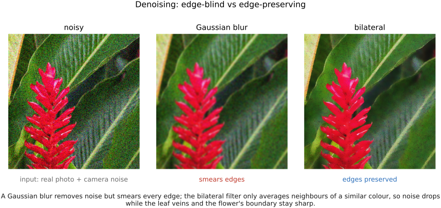
fig-denoising-before-after · denoising a real colour crop (realistic shot+read noise): noisy vs Gaussian (smears edges) vs bilateral (edge-preserving) (Denoising, BASIC)
fig-averaging-convergence
fig-averaging-convergence · averaging N noisy frames → noise drops as 1/√N (1, 3, 9, 25 frames), on a real colour photo with realistic shot+read noise (Denoising, BASIC)
4.16 Demosaicking
fig-demosaick-real-bayer
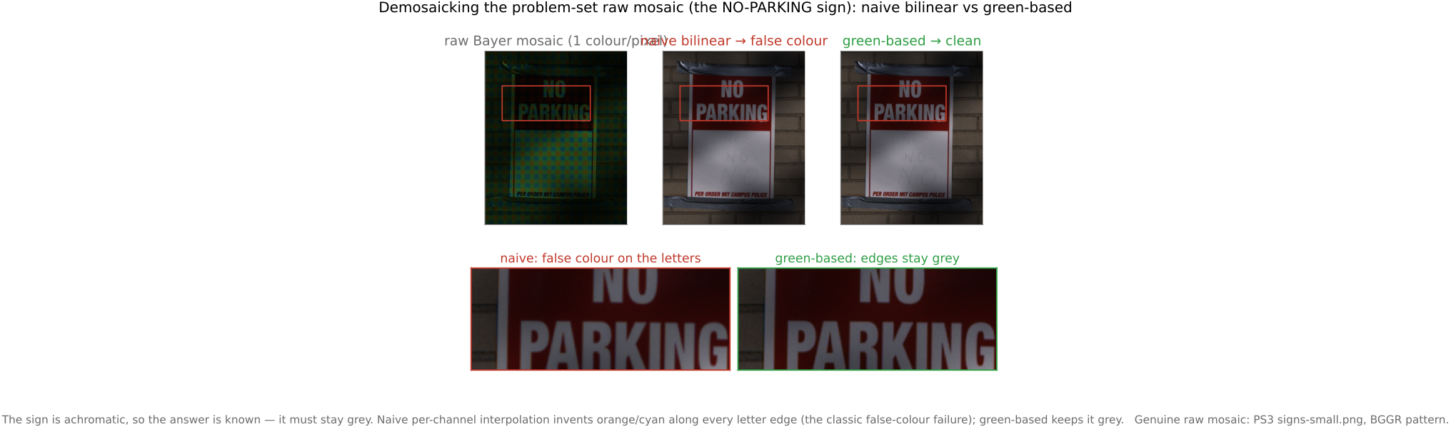
fig-demosaick-real-bayer · the PS3 raw mosaic (NO-PARKING sign) demosaicked: ground truth · simulated RGGB Bayer mosaic · naive bilinear (false colour on the window grid) · green-based (clean), with a zoom (Demosaicking, BASIC)
fig-demosaick-before-after
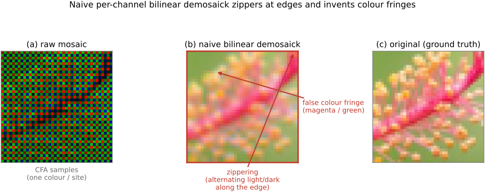
fig-demosaick-before-after · Bayer → RGB: the mosaic, naive bilinear demosaick (zipper / fringing), edge-aware (Demosaicking, BASIC) 🟨
4.16.2 Fuji X-Trans: a larger, irregular CFA
4.16.4 The task: full RGB at every pixel
4.16.10 Classic (non-learning) demosaicking: the general strategy
4.17 Auto-exposure and auto white balance
fig-ae-metering
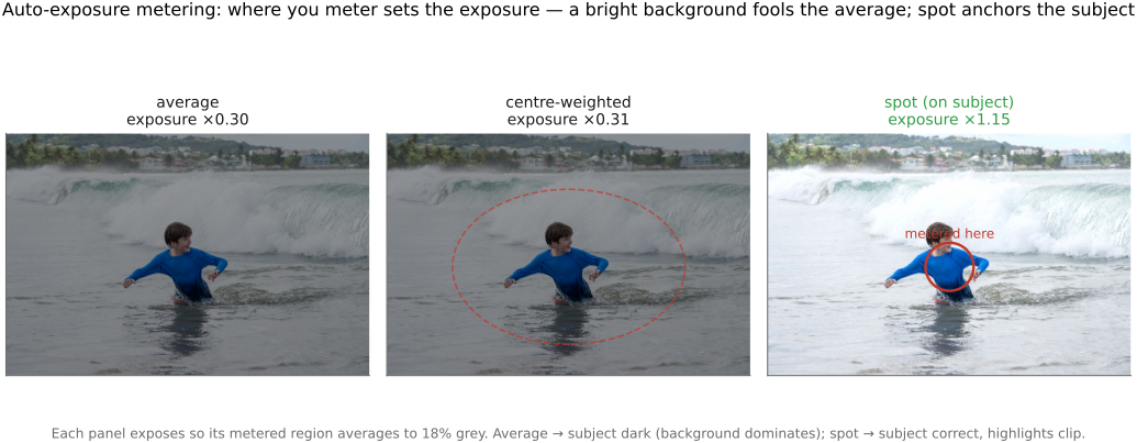
fig-ae-metering · **interactive** AE metering modes: pick a scene + mode (average / centre-weighted / movable+resizable spot); the demo exposes so the metered region averages 18% and reports metered tone, gain, and clipped %; "where you meter sets the exposure"
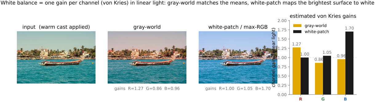
fig-white-balance-real
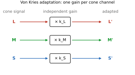
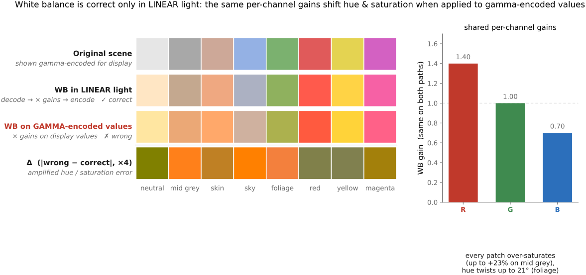
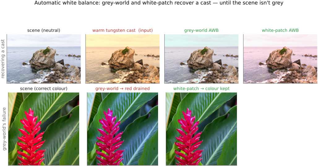
fig-white-balance-real · white balance computed from scratch (von Kries per-channel gain in linear light): a warm-casted photo corrected by gray-world vs white-patch/max-RGB, with the recovered channel gains (PS1)
4.18 File formats and compression
fig-jpeg-pipeline
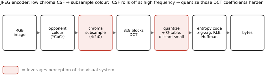
fig-jpeg-pipeline · the JPEG encoder — RGB → opponent colour → chroma subsample → 8×8 DCT → quantize → entropy code (File formats, BASIC) 🟨
fig-dct-basis
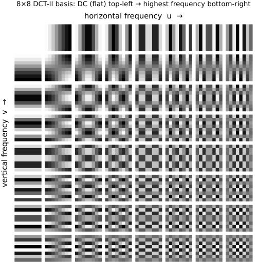
fig-dct-basis · the 8×8 DCT-II cosine basis (DC top-left → high frequency bottom-right) 🟨
fig-chroma-subsampling
fig-chroma-subsampling · chroma subsampling grids 4:4:4 / 4:2:2 / 4:2:0 (chroma sampled coarser than luma) 🟨
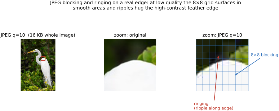
fig-jpeg-artifacts
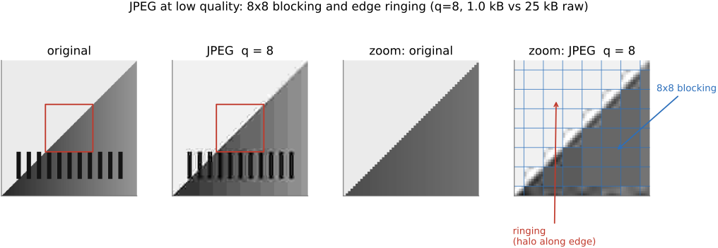
fig-jpeg-artifacts · JPEG blocking & ringing at low quality (original vs q=8, zoomed crop) 🟨
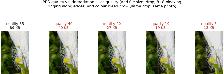
fig-jpeg-quality-levels
fig-jpeg-quality-levels · JPEG quality sweep (q=85→40→20→10→5): the same photo's edge-crop at each quality with the whole-image file size beneath — degradation grows as size drops (File formats, BASIC) 🟩
4.19 Recap ISP, non-destructive editing:
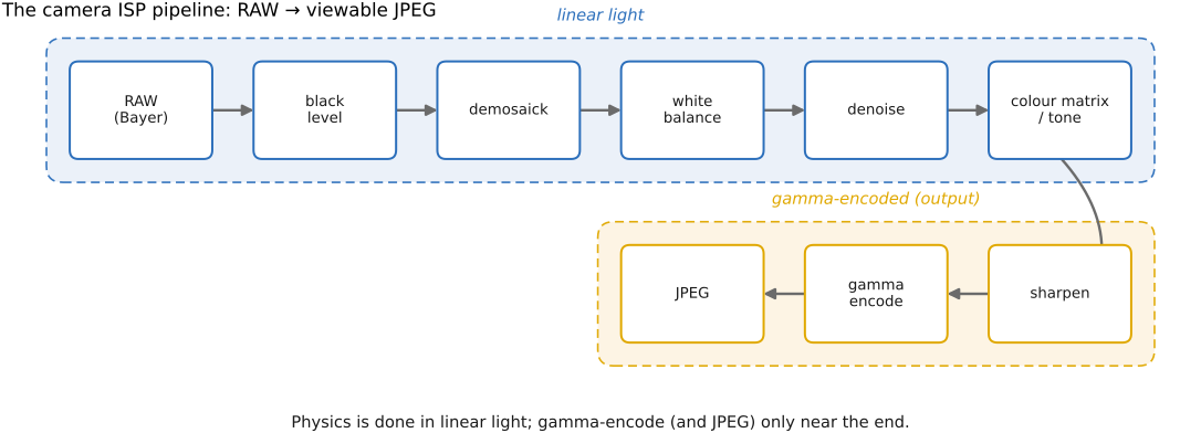
fig-isp-block-diagram
fig-isp-block-diagram · the ISP pipeline: RAW → black level → demosaick → white balance → denoise → tone/colour → sharpen → gamma → JPEG (Recap ISP, BASIC) 🟨
4.19.2 Pipeline design and tuning
4.19.3 The ISP, evolving: traditional → learned → generative
Part 5 COMPUTATIONAL TOOLS
The chapters before this one built images up from physics, perception, and the basic processing pipeline. This part assembles the **general-purpose computational tools** the rest of the book reaches for again and again: casting a recovery task as a **linear inverse problem** and solving it by regression; replacing a hand-designed operator with one **learned from data**; and **generating** plausible images with modern generative models. They are gathered here, before the single-image applications, because nearly every later part — deblurring, super-resolution, compositing, HDR, video — is at bottom an application of one of these three.
5.1 Linear Inverse Problems and Regression
fig-correspondence-then-transport
fig-correspondence-then-transport · the L17 spine — one scene displaced (two views / two faces / two frames / one long frame), each resolved by estimating a coordinate map (homography, morph field, flow, track, motion vector, camera path) then transporting pixels by one shared inverse-warp engine; the finding is hard, the moving is plumbing 🟨
fig-image-as-vector
fig-image-as-vector · an image *is* a vector: a 5×5 pixel grid unrolled into a tall column vector; n = H·W (Linear algebra) 🟩
fig-least-squares
fig-least-squares · line fit minimizing squared vertical residuals (Optimization & regression) 🟩
fig-deblur-preview
fig-deblur-preview · the deblur preview: sharp → blurred + noise → naive inverse amplifies noise; MTF 🟨
fig-gradient-descent
fig-gradient-descent · descent path on a convex-bowl contour (−∇f steps); too-large step overshoots (Optimization) 🟩
fig-pyramid-reconstruction
fig-pyramid-reconstruction · RECONSTRUCTION on a real photo: collapse the Laplacian pyramid coarse→fine (residual → +L_k each octave → exact image), plus an all-black per-pixel error panel (max ~1e-16 = lossless) (Reconstruction, BASIC)
fig-focus-stacking
fig-focus-stacking · optics-chapter illustrative figure (07-07 Figure 4): a stepped-focus stack → sharpness selection → all-in-focus composite. Synthetic per-slice defocus on one photo (`sourced/corn-cobs.jpg`, © Frédo Durand) — license-safe. The full real-data treatment lives in part-08 `fig-focalstack-*`
equations
forward model $y = Ax$
least squares $\hat x = \arg\min_x \tfrac12\|Ax - y\|^2$
normal equations $A^\top A\,x = A^\top y$
gradient of the data term $\nabla f(x) = A^\top(Ax - y)$
gradient step $x_{t+1} = x_t - \eta\,A^\top(Ax_t - y)$
convolution form $A x = k * x$ and $A^\top y = \tilde k * y$ (flipped kernel $\tilde k$)
per-frequency inverse $\hat x(\omega) = \hat y(\omega)/\hat k(\omega)$ (when it diagonalizes)
5.1.5 Efficient solvers
5.2 Efficient solvers
fig-gradient-descent
fig-gradient-descent · descent path on a convex-bowl contour (−∇f steps); too-large step overshoots (Optimization) 🟩
fig-pyramid-reconstruction
fig-pyramid-reconstruction · RECONSTRUCTION on a real photo: collapse the Laplacian pyramid coarse→fine (residual → +L_k each octave → exact image), plus an all-black per-pixel error panel (max ~1e-16 = lossless) (Reconstruction, BASIC)
fig-focus-stacking
fig-focus-stacking · optics-chapter illustrative figure (07-07 Figure 4): a stepped-focus stack → sharpness selection → all-in-focus composite. Synthetic per-slice defocus on one photo (`sourced/corn-cobs.jpg`, © Frédo Durand) — license-safe. The full real-data treatment lives in part-08 `fig-focalstack-*`
The previous chapter cast recovery as the normal equations $A^\top A\,x = A^\top y$ and made the key point that we **never build $A$** — every solver needs only to *apply* the blur and its transpose. This chapter is the toolkit that actually does the solving: a handful of matrix-free, iterative / multiscale methods, and the rule for which one to reach for. The same machinery returns in [[Poisson image editing]], colorization, matting, and gradient-domain HDR — learn it once here.
equations
matrix-free operator pair $A x = k * x$, $A^\top y = \tilde k * y$
gradient step $x_{t+1}=x_t-\eta\,A^\top(Ax_t-y)$
preconditioned CG ($M\approx(A^\top A)^{-1}$)
FFT one-shot $\hat x(\omega)=\hat y(\omega)\,\overline{\hat k(\omega)}/\big(|\hat k(\omega)|^2+\lambda|\hat L(\omega)|^2\big)$
5.3 Information theory
5.4 Fundamental limits of inverse problems
fig-inverse-conditioning
fig-inverse-conditioning · 1-D deconvolution: true signal · blurred+noisy measurement · singular-value spectrum decaying to the noise floor · naive inverse explodes · regularized inverse recovers
fig-lens-optimizer-demo
fig-lens-optimizer-demo · **interactive** unified lens-design optimizer (9.3 Lens optimization): orbitable 3-D lens (surfaces of revolution, Three.js) with a cone of rays arriving + converging on the sensor, a 2-D meridional slice of the same rays, on-axis/off-axis spot diagrams (true 2-D scatter, R/G/B chromatic) + a sensor close-up; stack ≤5 elements (n / R₁ / R₂ / position / dispersion); Run-optimizer = damped least squares (Levenberg–Marquardt) + basin-hopping over 3 fields × 7 wavelengths, sign-free curvature; replay slider + merit plot; spot/close-up scales locked during a run
fig-motion-blur-calculator
fig-motion-blur-calculator · live motion-blur calculator: a 3-D scene (walking figure or a car) imaged by a virtual camera, the blur rendered by **temporal supersampling** (many instants across the exposure, averaged). Set resolution / sensor / focal length (35 mm-equiv) / distance / exposure, add camera-shake **rates** in rotation (pitch/yaw/roll) and translation (x/y/z) plus a subject speed; the readout gives the blur at the subject in world (cm/m/in) and screen (px / % width) units, broken down by source. A per-pixel **G-buffer** (depth + subject mask) drives exact motion-vector arrows and a blur-magnitude heatmap: the subject carries its own motion, the background only camera shake. Environment backdrops + car colour picker. Static fallback is a screenshot. *3D models generated with Meshy AI.*
fig-focus-stacking
fig-focus-stacking · optics-chapter illustrative figure (07-07 Figure 4): a stepped-focus stack → sharpness selection → all-in-focus composite. Synthetic per-slice defocus on one photo (`sourced/corn-cobs.jpg`, © Frédo Durand) — license-safe. The full real-data treatment lives in part-08 `fig-focalstack-*`
fig-focalstack-capture
fig-focalstack-capture · a focus stack — several frames of one scene focused at different distances, the sharp slab moving through depth — plus an inset on refocusing the lens vs translating on a rail 🟨
💡 **Big lesson (L5.4, as a limit — the data is silent in the null space, and a prior only *invents* there):** an inverse problem can only return what the measurement actually constrained. Where the forward operator $A$ erased information (its null space) or barely kept it (near-null, noise-swamped modes), **no estimator can recover the truth** — the Cramér–Rao bound floors the variance, the data-processing inequality forbids manufacturing information, and the SVD names exactly which modes are lost. A prior (Tikhonov, sparsity, a learned/diffusion model) is the *only* thing that can fill those modes, and what it fills in is **plausible, not measured** — invented from training, not read from this photo. So progress comes in exactly two honest forms: **bring a better prior** (push the wall, accept invention) or **change $A$ at capture** (coded aperture, more exposures, structured light — so the wanted detail is measured in the first place). "AI enhance" is the former wearing the costume of the latter. (Registered in [[Big Lessons]] as the limit-form of **L5.4**; first stated in [[Image priors]] / FUNDAMENTALS, sharpened to an impossibility here.)
equations
forward model with noise $y = Ax + n$
**SVD** $A = U\Sigma V^\top$, reconstruction $\hat x = \sum_i \tfrac{u_i^\top y}{\sigma_i} v_i$ — modes with $\sigma_i\to 0$ are the **null/near-null space**, where the $1/\sigma_i$ factor explodes noise
**condition number** $\kappa(A)=\sigma_{\max}/\sigma_{\min}$
**Picard condition** (a stable solution needs $|u_i^\top y|$ to decay faster than $\sigma_i$)
**Tikhonov filter** $\hat x = \sum_i \tfrac{\sigma_i}{\sigma_i^2+\lambda}(u_i^\top y)\,v_i$ (the prior **damps** the explosive modes — and thereby **biases** them)
**Cramér–Rao** $\operatorname{Var}(\hat\theta) \ge 1/\mathcal I(\theta)$, Fisher information $\mathcal I$
**data-processing inequality** $I(x
y)\ge I(x
g(y))$ for any processing $g$
**resolution–noise / bias–variance** $\text{MSE}=\text{bias}^2+\text{variance}$.
5.4.1 The question: what can no algorithm recover?
5.4.2 The SVD picture: null space, near-null, and the noise explosion
5.4.3 Information bounds: a floor no estimator beats
5.4.4 The resolution–noise tradeoff, and how a prior invents
5.4.5 Fundamental versus practical, and coded capture as the escape
5.5 Machine learning
fig-learned-vs-handdesigned
fig-learned-vs-handdesigned · same inverse-problem skeleton, prior swapped: classical (data-fit + hand prior $\Phi$) vs learned ($f_\theta$ fit to data) (ML)
fig-synthetic-data-pipeline
fig-synthetic-data-pipeline · manufacture (degraded, clean) training pairs by simulating the camera/degradation (ML)
reference the ML & deep-learning refresher ([[Refreshers#Machine learning and deep learning]]) up front; this chapter does **not** re-teach networks — it sets up *learning an operator from data* and the **data** that powers it. The concrete deep-network operators are the next chapter, [[Deep learning]].
equations
learned operator $\hat I = f_\theta(\text{measurement})$ trained by $\min_\theta \sum_i \ell\!\big(f_\theta(x_i),\,y_i\big)$
reuse the inverse-problem $\hat I=\arg\min_I \lVert AI-b\rVert^2+\lambda\,R(I)$ from above to contrast a hand-tuned $R$ vs a learned one
5.6 Deep learning
fig-learned-task-zoo
fig-learned-task-zoo · learned low-level operators: denoise / super-resolve / demosaick / colorize, each input→output on one photo (ML)
fig-colorization-classical-vs-learned
fig-colorization-classical-vs-learned · Levin 2004 scribble-propagation vs Zhang 2016 fully-automatic colorization (ML)
⬜ figure not yet created
fig-depth-anything (one photo → its monocular depth map) fig-depth-anything
fig-gan-pix2pix
fig-gan-pix2pix · paired image-to-image translation: edge map → photo (conditional GAN) (ML)
fig-perceptual-metric
fig-perceptual-metric · same MSE, very different perception (small shift vs additive noise) → why LPIPS (ML)
these are the **deep-network** realizations of the learned-operator framing ([[Machine learning]]); architectures and training are the Refreshers' job — here we survey *what gets learned*.
equations
minimal (survey chapter) — perceptual / feature loss $\ell_{\text{feat}}=\sum_l \lVert \phi_l(\hat I)-\phi_l(I)\rVert^2$ over deep features $\phi_l$ (LPIPS)
reuse the learned operator $\hat I = f_\theta(\text{measurement})$ from [[Machine learning]]
5.7 Generative AI and diffusion
fig-genai-evaluate-vs-sample
fig-genai-evaluate-vs-sample · the generative leap (L5.2): a prior you can only *evaluate* ($\Phi$/denoiser) vs one you can *sample* ($x\sim p(x)$) (GenAI)
fig-diffusion-forward-reverse
fig-diffusion-forward-reverse · the two chains: forward $q$ adds Gaussian noise to a real photo; reverse $p_\theta$ denoises back (GenAI)
fig-diffusion-demo
fig-diffusion-demo · live interactive demo (web edition): type a prompt and watch the reverse process denoise from noise, step by step; static fallback is a noise→photo filmstrip (GenAI)
fig-score-is-denoiser
fig-score-is-denoiser · Tweedie: the score = the denoiser's correction toward the data manifold; one arrow, two names (GenAI)
fig-latent-diffusion
fig-latent-diffusion · encode → diffuse in a compressed latent → decode; prompt conditions by cross-attention (Stable Diffusion) (GenAI)
fig-posterior-sampling
fig-posterior-sampling · generative priors for inverse problems: one degraded $y$ → many plausible samples $x\sim p(x\mid y)$ (GenAI)
fig-conditioning-controlnet
fig-conditioning-controlnet · one prompt + a spatial hint (edges / pose / depth) → a generated image obeying both (GenAI)
This chapter is the **generative limit** of the two before it. *Machine learning* replaced a hand-designed prior with a **learned** one (L5.3); *Super-resolution* showed the prior is **not optional** and that a **denoiser is a universal prior** you can plug into any solver (L5.4, PnP/RED, and the punchline that the **score is a denoiser**). Here that same prior becomes something you can **sample from** — a generative model — and the canonical one, **diffusion**, is literally that denoiser run in a loop. We reference the ML / deep-learning refresher ([[Refreshers#Machine learning and deep learning]]) for U-Nets, transformers, and attention; this chapter does **not** re-teach networks — it surveys the *generative* idea and where it plugs back into the book's inverse-problem spine.
equations
forward (noising) process $x_t = \sqrt{\bar\alpha_t}\,x_0 + \sqrt{1-\bar\alpha_t}\,\epsilon$, $\epsilon\sim\mathcal N(0,I)$
training loss (predict the noise) $\mathbb{E}_{x_0,\epsilon,t}\big\lVert \epsilon - \epsilon_\theta(x_t, t)\big\rVert^2$
Tweedie / score = denoiser $\hat x_0 = x_t + \sigma_t^2\,\nabla_{x_t}\log p_{\sigma_t}(x_t)$, i.e. the score and a Gaussian denoiser are the same object
reverse (sampling) step — denoise a little, add a little noise, repeat from $x_T\sim\mathcal N(0,I)$ down to $x_0$
classifier-free guidance $\tilde\epsilon_\theta = \epsilon_\theta(x_t,\varnothing) + w\,\big(\epsilon_\theta(x_t,c) - \epsilon_\theta(x_t,\varnothing)\big)$
posterior sampling for an inverse problem — sample $x\sim p(x\mid y)\propto p(y\mid x)\,p(x)$ by alternating the diffusion prior step with a data-fit step against the forward model $A$ (a PnP/RED solver with a generative prior)
5.8 Image priors
fig-pnp-loop
fig-pnp-loop · Plug-and-Play / RED: alternate a data-fidelity step with a denoiser-as-prior step until convergence — the prior is a black-box denoiser 🟨
fig-denoiser-as-prior-spectrum
fig-denoiser-as-prior-spectrum · one PnP/RED prior slot, ever-stronger denoisers: hand-built → classical → learned → diffusion score (GenAI / Super-res)
equations
PnP iteration (HQS form) — alternate a **data-fit** step $z \leftarrow \arg\min_x \tfrac{1}{2}\lVert Ax - y\rVert^2 + \tfrac{\rho}{2}\lVert x - \tilde{x}\rVert^2$ and a **denoise** step $\tilde{x} \leftarrow \mathcal{D}_\sigma(z)$ (the prior, *any* denoiser $\mathcal{D}$)
RED gradient $\nabla \Phi(x) = x - \mathcal{D}(x)$ (prior gradient = residual of a denoiser)
Tweedie $\hat{x} = z + \sigma^2\, \nabla_z \log p_\sigma(z)$ (the score IS a Gaussian denoiser → diffusion = iterated $\mathcal{D}$)
Part 6 EDGES MATTER
The thread of this part is that **where the edges are** governs the edit. Edges carry most of an image's meaning, so three families of method are organised around them: **gradient-domain (Poisson) editing** reconstructs an image *from* its edges (seamless cloning, gradient-domain HDR, photomontage); **edge-preserving filtering** smooths everything *except* across edges (bilateral, guided, local Laplacian, non-local means → tone mapping, detail, denoising); and **seam optimization** cuts *along* the least-noticeable edges (seam carving, graph-cut compositing). All three lean on the linear-systems and convolution machinery from earlier parts; they belong together because they share one idea — respect the edges.
6.1 Bilateral filtering
6.2 Non-local means
fig-nlmeans-patches
fig-nlmeans-patches · non-local means: compare *patches* not pixels — similar patches elsewhere vote for the centre pixel (NL-means)
⬜ figure not yet created
interactive weight-map demo [fig-nlmeans-demo] fig-nlmeans-demo
• chapter intro: split out of [[Denoising]]; NL-means is the bilateral filter living in patch space, and the reason image self-similarity denoises so well.
6.3 Edge-preserving optimization — colorization
• **the shift — filtering → optimization**: instead of one weighted-average *pass*, solve a **global least-squares** problem whose smoothness term uses the affinity as a weight. The same affinity, now inside an energy.
• **colorization** (the demo): the user scribbles a few colors; **propagate** them so that **neighbouring pixels of similar luminance get similar color** — minimize $\sum_p (U_p-\sum_{q\in N(p)} a_{pq} U_q)^2$ over the chrominance $U$, with affinity $a_{pq}$ **large where $I_p\approx I_q$** (small luminance difference) — exactly the bilateral's range idea inside a quadratic energy
• **solve it** with the linear-systems machinery of the regression chapter — sparse, structured, solved by CG / multigrid (cross-ref [[Single-image computational photography#Blind deblurring]], [[Linear Inverse Problems and Regression]])
• the **affinity matrix** here is the same object as the **matting Laplacian** and the graph-cut edge weights → forward-ref [[#Compositing, segmentation and matting]] (matting / segmentation = affinity again)
• also placeable under [[Single-image computational photography#Blind deblurring]] (the "Colorization as optimization?" stub) — keep the *technique* here, cross-ref from there
6.3.1 The shift: filtering becomes optimization
6.3.2 Colorization: the canonical demonstration
6.3.3 Writing down the energy
6.3.4 Solving it: a sparse linear system we already own
6.3.5 One affinity, two faces: the matting Laplacian connection
6.4 Local Laplacian filters
⬜ figure not yet created
`fig-exposure-fusion-mertens` [candidate] — a 3-shot exposure bracket + its three per-pixel quality-weight maps (contrast · saturation · well-exposedness) → the **Laplacian-pyramid-blended** fused image, sharp and halo-free, *with no HDR radiance map ever formed* fig-exposure-fusion-mertens
fig-local-laplacian
fig-local-laplacian · local Laplacian filters on a real HDR sunset (Paris–Hasinoff–Kautz 2011, implemented from scratch): naive global (blown) vs Gaussian base (halo) vs local Laplacian (halo-free) tone mapping, plus the compressive remapping curve $r_g(\cdot)$ (detail centre + identity tails) and a zoom comparison proving the silhouette stays halo-free (Local Laplacian filters)
⬜ figure not yet created
before/after detail-boost with **no halo** fig-wb-before-after
• **start here — Mertens *exposure fusion*, the gentlest pyramid method**: the cleanest way into this chapter is the technique that does **local tone mapping for free, without ever building an HDR image or choosing a tone curve**. Given a **bracketed stack** (or several renderings of one scene), score each pixel of each frame by simple **quality weights** — **contrast** (Laplacian magnitude, "is it sharp here?"), **saturation** (spread of the RGB channels, "is the color alive?"), and **well-exposedness** (closeness to mid-grey, "is it neither crushed nor blown?") — then keep, per pixel, the best-exposed frame. *(Mertens, Kautz & Van Reeth 2007.)* [`fig-exposure-fusion-mertens`]
• **the catch, and the fix — blend in the Laplacian pyramid**: a *per-pixel* weighted average of the frames **seams and halos** (the weights jump at boundaries between which frame "wins"). The fix is **pyramid blending** ([[Pyramids and wavelets]], Burt–Adelson): build a **Laplacian pyramid of each frame** and a **Gaussian pyramid of each (normalized) weight map**, blend the coefficients **level by level** (each frequency band fused at its own scale, with a correspondingly-blurred weight), then collapse. Because every band is feathered over a scale-appropriate transition, the join is invisible and no halos appear — the same reason pyramid blending hides a seam, now driven by exposure-quality weights.
• **why it opens the chapter**: it is the most intuitive instance of the chapter's one idea — *do the edge-aware / local-tone work **band-by-band in a Laplacian pyramid**, not pixel-by-pixel* — and it needs no range weight, no base/detail split, no radiance map. (Full HDR-capture context and where exposure fusion sits among merge-then-tonemap pipelines: [[Multiple exposure imaging]]; here it is the on-ramp to the pyramid machinery.)
• **from fusing a stack to reshaping one image — local Laplacian filters**: exposure fusion *blends several images* in the pyramid; **local Laplacian filters** (Paris et al. 2011) take the same "manipulate the Laplacian pyramid, halo-free" idea and apply it to a **single** image, reshaping its own bands by a pointwise remapping. Same home (the Laplacian pyramid), one input instead of a stack.
• **the odd one out — not an affinity method**: every other technique here weights *pairs* of pixels by similarity; local Laplacian instead works **band-by-band in a Laplacian pyramid** with a **pointwise remapping** — no range weight, no base/detail split (so none of the halos / gradient reversals those can produce). The multiscale cousin of the bilateral, by a different mechanism. Cross-ref [[Pyramids and wavelets]] (the pyramid it's built on) and [[Bilateral filtering]].
• **the mechanism**: to compute the output's Laplacian coefficient at a pixel and level, take the pixel's value $g$, apply a **remapping function** $r_g(\cdot)$ to the *whole* image (a smooth curve, centred on $g$, that decides what is "detail" vs "edge"), build a Laplacian pyramid of that remapped image, and read off **just this level's coefficient at this pixel**; collapse the resulting pyramid for the result.
• **the knob is the remapping $r$**: near $g$ (small amplitude = **detail**) it **compresses or amplifies** — controlling detail / local contrast; far from $g$ (large amplitude = **edge**) it stays the **identity** — so strong edges pass through untouched. One curve → detail enhancement, tone mapping, or inverse tone mapping, all **artifact-free**.
• **why it matters**: state-of-the-art **edge-aware detail manipulation and HDR tone mapping** with no halos and no gradient reversal — the failure modes that motivated the bilateral in the first place.
• **cost & the fast version**: the naive form rebuilds a pyramid per pixel-and-level (expensive); **Aubry et al. 2014** gives a fast approximation and shows the **unnormalized bilateral** is its single-scale relative (ties back to [[Bilateral filtering#Bilateral filter|the unnormalized bilateral]]).
6.4.1 The wish, and why the bilateral leaves a halo
6.4.2 What a Laplacian pyramid hands you
6.4.3 The mechanism: a remapping recomputed per output pixel
6.4.4 One curve, three edits: enhancement, tone mapping, inverse tone mapping
6.4.5 Contrast with the bilateral base/detail split
6.4.6 The cost, and the fast version
6.5 Matting Laplacian
6.6 Guided image filtering
• **the idea**: like the joint bilateral (filter $I$, take structure from a **guide** $J$) but the output is a **local linear transform of the guide**, $I^{\mathrm{out}}=a_k J + b_k$ fit per window by **least squares** — so it preserves the guide's edges by construction
• **why prefer it**: **$O(N)$**, **no range-quantization artefacts** (the gradient reversal the bilateral can show), and **differentiable** → drops into learning pipelines
• **uses**: edge-preserving smoothing; detail enhancement; **flash / no-flash**; **matting / feathering**; **dehazing** (guide = the hazy image — xref He, Sun & Tang 2009 dark-channel, [[#Dehazing as a prior-driven inverse problem]]); depth upsampling
• the affinity is now **implicit** in the local linear fit — same family, different mechanism; a fitting end-point for the chapter's through-line (bilateral → grid → learned → regression → optimization → guided, all *affinity*)
6.6.1 The key idea: the output is a local line in the guide
6.6.2 Fitting the line, and the one knob
6.6.3 Why it is fast: O(N) regardless of window size
6.6.4 No gradient reversal
6.6.5 Reading the affinity back out
6.6.6 Where it is used
6.7 Locally adaptive regression kernel (LARK)
• **the view**: treat denoising / upsampling as **local regression** — fit a smooth function to nearby pixels, weighted by a kernel
• **steering / adaptive kernels**: shape the kernel to the **local image structure** — estimate the local gradient, then **stretch the kernel *along* edges and squeeze it *across* them** (an anisotropic, data-dependent weight) so it averages along the edge, not across it
• so LARK is the **regression flavour** of the same affinity idea: the kernel geometry is *derived from* local structure, generalizing the bilateral's scalar range weight to an oriented one
• also a **descriptor**: LARK signatures are used for detection / matching (Seo & Milanfar) — note in passing, not developed
6.7.1 Change the verb: from averaging to fitting
6.7.2 Steering the kernel to the local structure
6.7.3 The regression flavour of the affinity
6.7.4 LARK as a structure descriptor
6.8 Poisson image editing
fig-seamless-cloning
fig-seamless-cloning · Poisson seamless cloning (Pérez 2003), EDGES MATTER → Poisson editing: a disk of Jupiter cloned onto Earth — destination (target ring) · source patch · naive paste (visible ring) · Poisson paste (seam gone)
fig-gradient-domain-pipeline
fig-gradient-domain-pipeline · gradient-domain (Poisson) workflow: image → take gradients (∇f) → modify the field → integrate by solving ∇²f=div v → reconstructed (EDGES MATTER → Poisson editing)
fig-mixing-gradients
fig-mixing-gradients · mixing gradients — keep the per-pixel *stronger* gradient so destination texture shows through holey / transparent inserts (naive vs max-gradient paste) (Poisson editing)
⬜ figure not yet created
`fig-chong-colorspace-results` — results from Chong, Gortler & Zickler 2008 [placeholder] fig-chong-colorspace-results
fig-poisson-vs-laplacian-blend
fig-poisson-vs-laplacian-blend · Poisson vs Laplacian-pyramid blending, contrasted on the DC: 1-D three cases (matched level — both agree; mismatched pedestal — Poisson re-lights, pyramid leaves a halo; constant — Poisson ramps/dissolves, pyramid keeps a feathered plateau) + 2-D (paste a constant square — Poisson dissolves it via the harmonic membrane, pyramid keeps a feathered version)
fig-poisson-fourier
fig-poisson-fourier ·
equations
the **Poisson equation** $\nabla^2 f = \operatorname{div}\mathbf{v}$ (reconstruct the field $f$ whose gradient best matches guidance $\mathbf{v}$)
the **discrete Laplacian** system $4f_{p}-\sum_{q\in N(p)} f_{q}=\sum_{q\in N(p)}\!\big(\,v_{pq}\,\big)$ (one sparse equation per pixel $p$ over its 4-neighbours $N(p)$)
the **seamless-cloning Dirichlet boundary condition** $f|_{\partial\Omega}=f^{*}|_{\partial\Omega}$ (interior gradients from the source, boundary values pinned to the destination $f^{*}$)
6.8.4 A perception-based color space
6.8.7 Screened Poisson: pinning the low frequencies
6.8.9 Decolorization (Color2Gray) — keeping isoluminant contrast
6.9 Seam optimization
• **the third leg of EDGES MATTER** (the part's framing payoff): Poisson **reconstructs from edges**, bilateral **smooths except across edges**, seam optimization **cuts along edges**. State it as the dual of edge preservation: edge-preserving filtering works *hard to avoid* edges; seam methods *go looking for them* — a transition is invisible exactly where the image is already changing, so we hide the cut **in the edges / busy texture** and keep it **out of smooth regions** where a seam would scream. (Callback to the part intro's "respect the edges.")
• the **unifying machinery**: all three sub-families are **discrete optimization on a graph or grid** — a 1-D least-cost path (**DP**), a 2-D globally-optimal boundary (**graph cut / min-cut**), or a spectral partition (**normalized cuts**). What changes between methods is **the energy / affinity**, not the optimizer.
💡 **Big lesson:** *many image edits are **discrete optimization on a graph** — dynamic programming, min-cut/max-flow, or spectral relaxation — and the **energy (affinity) you choose is the whole game**.* The optimizer is off-the-shelf; **what** you penalize (gradient magnitude, label disagreement across edges, region/boundary cost) is the design. This is the **L4.21 affinity** principle (Bilateral) turned into a *cut*: there the affinity said "average these together"; here it says "**don't cut here**." *(Register as new lesson **L6.4 · Image edits as discrete optimization on a graph (the energy is the design)**, first appearance here; "also relevant": Poisson/photomontage, compositing/segmentation/matting, texture synthesis, stereo/MRF labeling. Full box at this section's head; one-line callback to L4.)*
6.9.5 GrabCut — interactive cutout from a single rectangle
6.10 Recap: which edge-aware technique when?
fig-edge-aware-taxonomy
fig-edge-aware-taxonomy ·
6.10.3 A worked chooser
Part 7 WARPING, MORPHING, AND LAGRANGIAN APPROACHES
💡 **Big lesson (L17 · transport half):** almost every geometric technique is **(1) establish a correspondence / coordinate map**, then **(2) transport pixels along it** by warping and resampling. This part owns step (2) — one shared engine serving rectification, panoramas, morphing, stabilization, and frame interpolation — and the ways to *build* a map from sparse control. The hard *estimation* half (step 1) is [[Matching pixels across space and time]].
7.1 Warping
fig-warp-domain-vs-range
fig-warp-domain-vs-range · one image, two orthogonal arrows — the domain arrow bends the grid (a pixel slides, carrying its colour; a warp), the range arrow recolours in place (a point/tone op); warping moves where, not what 🟨
⬜ figure not yet created
`fig-forward-warp-holes` (forward/input-driven warp scatters input pixels to fractional output locations → gaps (uncovered output) and pile-ups (many inputs to one output)) fig-forward-warp-holes
fig-inverse-warp-lookup
fig-inverse-warp-lookup · inverse (output-driven) warping, the useful idiom — loop over output pixels, push each back through $f^{-1}$, sample there; every output covered once, the only difficulty a clean resampling 🟨
fig-recon-filters-1d
fig-recon-filters-1d · nearest (boxy staircase), linear (kinked through every sample), and cubic (smooth with mild overshoot) reconstruction of the same 1-D sample row — the sharpness/smoothness trade 🟨
⬜ figure not yet created
`fig-bilinear-weights` (the four surrounding pixels and the fractional-coordinate area weights of bilinear interpolation) fig-bilinear-weights
fig-minify-aliasing-moire
fig-minify-aliasing-moire · the L16 picture — a fine grating decimated naively (folds into false moiré) vs area-averaged first then decimated (clean); same size, opposite outcomes, decided by prefiltering 🟨
⬜ figure not yet created
`fig-kernel-scaling-minify` (the reconstruction kernel widened by the downscale factor so it averages over the right footprint — "gather farther when shrinking") fig-kernel-scaling-minify
fig-dof-ladder
fig-dof-ladder · the degrees-of-freedom ladder — a unit square under translation (2) → similarity (4) → affine (6) → projective (8) → free-form ($\infty$), each rung breaking a preserved property 🟨
fig-mesh-triangulation-warp
fig-mesh-triangulation-warp · piecewise-affine mesh warp — control matches triangulated, each triangle carrying its own affine map; exact and fast but only $C^0$, creasing along shared edges 🟨
⬜ figure not yet created
`fig-tps-rbf-warp` (a few control points displaced → a smooth thin-plate-spline field filling the gaps, minimal bending) fig-tps-rbf-warp
fig-beier-neely-segments
fig-beier-neely-segments · Beier–Neely feature-line warp — before/after directed segments, one segment's $(u,v)$ frame, and the distance-weighted blend of several segments' proposed displacements ($w_i=(\ell_i^p/(a+d_i))^b$) 🟨
fig-arap-vs-affine
fig-arap-vs-affine · drag one handle — an unconstrained affine/least-squares warp shears and stretches, vs an as-rigid-as-possible / MLS warp that keeps each neighbourhood near a rotation so the shape bends without stretching
💡 **Big lesson (L16 · Prefilter before you downsample):** a warp that *shrinks* the image (minifies) is throwing samples away — and if you just decimate (keep every $N$th source pixel, or sample a narrow reconstruction kernel) the detail too fine for the new grid **folds down into bold false moiré**, not into nothing. The fix is to **area-average first**: widen the resampling kernel in proportion to the downscale factor $s$ (so it gathers over the whole footprint each output pixel now covers) and renormalize — that low-pass blur is the prefilter. Enlarging needs *no* prefilter (clamp the kernel width to 1); shrinking *always* does. (→ see Big lesson **L16**, first placed in BASIC → Resampling; the frequency-domain *why* is **L4.8** — aliasing folds frequencies above the new Nyquist. The same lesson governs every geometric resample in this part: rectification corners that shrink, stabilization crops, optical-flow rendering.)
⚠️ **Candidate new part-spine lesson (flag only — not registered).** Almost every algorithm in this part follows one shape: **establish a correspondence / coordinate map between two images (or an image and a target frame), then transport pixels along it.** Warping makes the map explicit and applies it; perspective rectification *solves* the map (a homography) from constraints; panorama stitching *estimates* the map from features; morphing *interpolates between* two maps; optical flow *estimates a dense map* from brightness constancy; stabilization *smooths a map over time*; frame interpolation *renders along* a map. A lesson like **"find the coordinate map, then move the pixels"** would unify the part the way L5.4 unifies the inverse-problem part. Worth registering as a part-spine lesson for MOTION/WARPING — *noted here, deliberately not registered* (registry-first convention: register in [[Big Lessons]] before placing).
equations
warp as a domain map $\text{out}(x,y)=\text{in}\big(f^{-1}(x,y)\big)$ (move the domain, keep the range)
**forward** warp $\text{out}(f(x,y))\leftarrow \text{in}(x,y)$ (scatters → holes)
1-D **linear** reconstruction $\text{im}(x)= (1-\alpha)\,\text{im}[\lfloor x\rfloor]+\alpha\,\text{im}[\lceil x\rceil]$, $\alpha=x-\lfloor x\rfloor$
**bilinear** = separable 1-D linear in $x$ then $y$ (four-neighbour area weights)
general **convolution resampling** $\text{out}(x)=\sum_{x'}k\big(f^{-1}(x)-x'\big)\,\text{in}(x')$ with analytic kernel $k$ centred at the fractional source location
**minification kernel scaling** $k_s(t)=\tfrac1s\,k(t/s)$ for downscale factor $s$ (widen + renormalize → area-average = prefilter, **L16**)
**affine** $\begin{psmallmatrix}x'\\y'\end{psmallmatrix}=A\begin{psmallmatrix}x\\y\end{psmallmatrix}+\mathbf t$ (6 DOF)
**projective / homography** $\begin{psmallmatrix}x'\\y'\\w'\end{psmallmatrix}=H\begin{psmallmatrix}x\\y\\1\end{psmallmatrix}$, then $(x'/w',y'/w')$ (8 DOF
solve from 4 correspondences — [[Manual panorama stitching from multiple views]])
**TPS / RBF** field $f(\mathbf p)=A\mathbf p+\mathbf t+\sum_i w_i\,\phi(\lVert\mathbf p-\mathbf c_i\rVert)$ with $\phi(r)=r^2\log r$ (thin-plate radial basis)
**Beier–Neely** single-segment map via the segment frame $u=\dfrac{(\mathbf X-\mathbf P)\cdot(\mathbf Q-\mathbf P)}{\lVert\mathbf Q-\mathbf P\rVert^2},\ v=\dfrac{(\mathbf X-\mathbf P)\cdot\perp(\mathbf Q-\mathbf P)}{\lVert\mathbf Q-\mathbf P\rVert}$, then $\mathbf X'=\mathbf P'+u(\mathbf Q'-\mathbf P')+\dfrac{v\,\perp(\mathbf Q'-\mathbf P')}{\lVert\mathbf Q'-\mathbf P'\rVert}$, multi-segment weight $w_i=\Big(\dfrac{\ell_i^{p}}{a+d_i}\Big)^{b}$.
7.1.3 Resampling — a quick reminder (developed in BASIC)
7.1.7 Liquify — the warp with a paintbrush bolted on
7.2 Antialiasing for complex transforms
fig-footprint-ellipse-jacobian
fig-footprint-ellipse-jacobian · one output-pixel circle back-projected through a perspective warp maps to a footprint ellipse; major/minor axes = singular values/vectors of the local Jacobian J (square only under a similarity); + a worked perspective grid
fig-isotropic-vs-anisotropic-floor
fig-isotropic-vs-anisotropic-floor · receding checkerboard floor filtered three ways: point (aliased moiré) / isotropic (over-blur) / anisotropic-EWA (crisp into distance)
fig-ewa-gaussian-ellipse
fig-ewa-gaussian-ellipse · elliptical-Gaussian EWA weight over source texels; conic Q≤F bounding box; incremental finite-difference march
fig-feline-probe-line
fig-feline-probe-line · footprint ellipse approximated by a line of N circular trilinear MIP probes along the major axis, each sized to the minor axis (16× anisotropic; trilinear = N=1)
fig-sat-ripmap
fig-sat-ripmap · summed-area table box average from 4 corner lookups of the integral image + ripmap grid of pre-shrunk-in-x/-in-y levels (axis-aligned anisotropy only)
💡 **Big lesson (L16, anisotropic):** the prefilter-on-minify discipline (**L16**) is *direction-dependent* the moment the warp stops being a similarity. A general warp compresses the source more along one axis than another, so the right prefilter is not a round blur but an **oriented ellipse** — average a lot along the compressed direction, barely at all across it. Isotropic filtering must then either alias the compressed axis or blur the sharp one; anisotropic filtering (EWA and its approximations) does both jobs at once. Same lesson, one dimension richer.
equations
**footprint Jacobian** $J=\partial f^{-1}/\partial(x,y)$ (local linearization of the inverse warp)
the unit screen circle → ellipse with **covariance** $\Sigma=JJ^{\!\top}$, radii the singular values $\sigma_1\ge\sigma_2$ of $J$, **anisotropy** $\rho=\sigma_1/\sigma_2$
**EWA conic / Mahalanobis form** $Q(\mathbf u)=\mathbf u^{\!\top}\Sigma^{-1}\mathbf u=Au^2+Buv+Cv^2$, weight $w=\exp(-\tfrac12 Q)$ for $Q\le F$ (an elliptical Gaussian)
**incremental evaluation** $Q(u{+}1,v)=Q(u,v)+(2Au+Bv+A)$ with the increment itself stepped by the constant $2A$ → ~2 adds/texel
**Feline** probe centres $\mathbf c_i=\mathbf c\pm t_i\,\hat{\mathbf e}_1$ along the major axis $\hat{\mathbf e}_1$, each a trilinear sample at level $\text{LOD}=\log_2\sigma_2$, Gaussian-weighted
**summed-area box** average $=\big(S(x_1,y_1)-S(x_0,y_1)-S(x_1,y_0)+S(x_0,y_0)\big)/\text{area}$ with $S$ the integral image
**max-anisotropy clamp** $\sigma_1\leftarrow\min(\sigma_1,\rho_{\max}\sigma_2)$.
7.3 Morphing
fig-morph-crossfade-ghost
fig-morph-crossfade-ghost · why a cross-dissolve ghosts — two misaligned faces averaged at $t=0.5$ superimpose features into a translucent four-eyed, two-mouthed ghost; the blend handled colour but ignored position
⬜ figure not yet created
the failure that motivates everything)
fig-morph-shape-vs-color
fig-morph-shape-vs-color · the two orthogonal knobs of a morph — range (colour) as the cross-dissolve and domain (shape) as feature-position interpolation; a true morph is their product, the square's corners labelling the four extremes 🟨
fig-morph-recipe
fig-morph-recipe · the three-step morph at $t=0.5$ — interpolate the features to the midpoint shape, warp both images to that same shape, then cross-dissolve; a sharp single face because alignment preceded the blend 🟨
⬜ figure not yet created
`fig-beier-neely-oneseg` (a single before/after line pair: the $(u,v)$ coordinate frame along/perpendicular to the segment, and how a point $X$ maps to $X'$) fig-beier-neely-oneseg
⬜ figure not yet created
`fig-beier-neely-multiseg` (several line pairs, each proposing an $X'_i$, combined by a distance/length **weighted average** — the field warp) fig-beier-neely-multiseg
fig-mesh-vs-field-morph
fig-mesh-vs-field-morph · two ways to drive the same morph — mesh (per-triangle affine, strictly local, fiddly, can crease) vs field/Beier–Neely (a few control lines, globally-supported distance-weighted field, sparse but fold-prone) 🟨
fig-view-morph-prewarp
fig-view-morph-prewarp · why two views need view morphing — a naive 2-D morph bends straight edges and shrinks a rotating object, vs view morphing (prewarp to aligned epipolar lines → interpolate → postwarp) keeping lines straight and shape intact 🟨
💡 **Big lesson (recurrence — *align before you blend*):** averaging two images only makes sense once their features sit at the *same place*. A plain cross-dissolve blends colors at fixed coordinates, so any misalignment **double-exposes into a ghost**; the cure is to **warp into correspondence first, then average** — the same move as panorama de-ghosting and multi-frame super-resolution's sub-pixel alignment. Morphing is this lesson taken to its limit: not just align-then-average, but interpolate the *alignment itself* over $t$. (Companion to the *capture-then-decide / align-then-merge* family; the dense automatic aligner is [[Optical flow]].)
7.4 Morphable models
7.4.1 Step 1 — dense correspondence: the precondition for averaging shapes
7.4.2 Step 2 — Procrustes alignment: factor out pose so PCA sees shape
7.4.3 Step 3 — PCA: a mean and a basis of eigen-deformations
7.4.4 Step 4 — shape and appearance are *separate* bases
7.4.5 Step 5 — fitting a new photo: analysis-by-synthesis
7.4.6 Step 6 — once fitted, edit by moving in the space
7.4.7 Step 7 — from linear PCA to neural priors
7.4.8 Recap and significance
7.5 Shape-preserving warping
7.5.1 Why plain interpolation shears: the rigidity gap
7.5.2 As-rigid-as-possible (ARAP) manipulation
7.5.3 Linear blend skinning and why the weights decide everything
7.5.4 Bounded biharmonic weights (BBW)
7.5.5 ARAP interpolation: rigid-as-possible morphing between two poses
7.5.6 Moving least squares: the simpler cousin
7.5.7 Recap and significance
7.6 Perspective distortion and its correction
fig-keystoning-cause
fig-keystoning-cause · keystoning is the tilt, not the lens — a camera tilted up makes world-parallel verticals converge (façade → trapezoid), while the fronto-parallel shot keeps them parallel; projection preserves lines, not parallelism 🟨
fig-rectify-before-after
fig-rectify-before-after · rectifying by homography — a keystoned input with four corner handles dragged onto a known rectangle (vanishing point marked) re-rendered fronto-parallel by $\text{out}(\mathbf x)=\text{in}(H^{-1}\mathbf x)$ 🟨
⬜ figure not yet created
`fig-vanishing-point-autosolve` (detected parallel-line bundles meeting at vanishing points → the homography that sends the vertical VP to infinity straightens the verticals) fig-vanishing-point-autosolve
fig-tilt-shift-scheimpflug
fig-tilt-shift-scheimpflug · fixing perspective in the lens — shift moves the sensor within an oversized image circle while staying parallel to the façade (no converging verticals), tilt sets the focus plane via the Scheimpflug condition 🟨
⬜ figure not yet created
`fig-rectify-resample-stretch` (the rectified output's non-uniform resolution: the far/top corners are enlarged and softened while the near edge is compressed — why one homography only rectifies a *plane*). fig-rectify-resample-stretch
💡 **Big lesson (L16 recurrence · prefilter the shrinking corners):** rectification does not resample uniformly — to make the *far* (top) of the façade as wide as the *near* edge, the homography **enlarges** the top corners (upsample → just interpolate) and **compresses** other regions (downsample → must prefilter, or alias). So a faithful rectifier applies the **prefilter-before-downsample** discipline *per region*, with the kernel footprint set by the **local Jacobian** of $H$ (how much each area shrinks). (→ see Big lesson **L16**, [[Warping]] / BASIC Resampling.)
equations
the rectifying map is a **homography** $\mathbf x' \simeq H\mathbf x$ (homogeneous
divide by $w'$) — the projective warp of [[Warping]]
solve $H$ from **4 correspondences** (building corners → target rectangle), each pair giving 2 linear equations, $H$ up to scale → 8 DOF (least squares / SVD, per [[Manual panorama stitching from multiple views]])
applied by **inverse warp + resample** $\text{out}(\mathbf x)=\text{in}\big(H^{-1}\mathbf x\big)$
the **auto** constraint: choose $H$ so the bundle of (imaged) parallel lines maps to a **vanishing point at infinity** (verticals become vertical / parallel).
7.6.4 A different perspective distortion — wide-angle portraits, and a content-aware fix
7.6.5 A montage has no single viewpoint — a family in a box
Part 8 MATCHING PIXELS AND HUMANS ACROSS SPACE AND TIME
💡 **Big lesson (L17 · estimation half):** correspondence-then-transport — this part owns the **hard, ill-posed estimation** half (where did each pixel go?), ill-posed by the **aperture problem** and broken by occlusion and large motion; [[Warping and morphing]] owns the transport. Matching is literally the inverse of warping: warping consumes a coordinate map, matching produces one.
8.1 Brute force
fig-align-before-average
fig-align-before-average · averaging an unregistered hand-held burst (a blurry double) vs averaging the same burst after alignment (sharp, clean, $1/\sqrt N$ benefit visible)
fig-ssd-search-surface
fig-ssd-search-surface · the SSD score over candidate $(dx,dy)$ shifts drawn as a single-welled basin whose minimum marks the true alignment 🟨
fig-phase-correlation-spike
fig-phase-correlation-spike · two shifted frames producing, via the inverse FFT of the normalized cross-power spectrum, a single sharp delta whose position is the inter-frame shift 🟨
⬜ figure not yet created
L4.8 in a picture)
fig-coarse-to-fine-pyramid
fig-coarse-to-fine-pyramid · alignment estimated cheaply at the coarsest pyramid level then propagated and refined down to full resolution, capturing large motions while avoiding local minima 🟨
fig-channel-align-sergey
fig-channel-align-sergey · translational alignment in the wild: Prokudin-Gorsky's three colour-separation plates stacked naively (colour fringes) vs registered by SSD/NCC shift search (clean)
💡 **Big lesson (L4.8 here · diagonalize when you can):** a pure translation is *diagonal* in the Fourier basis — it leaves every magnitude untouched and tilts only the phases by a ramp whose slope **is** the shift. So a brute-force $O(\text{window}^2)$ shift search collapses to a single FFT pair: form the normalized cross-power spectrum, inverse-transform, and read the shift off the location of the resulting delta. Whenever the operator is a shift, a convolution, or a correlation, ask first whether the frequency domain turns the work into a per-frequency (diagonal) operation. *(L4.8, first placed in [[Linearity, Fourier, aliasing and deblurring]]; here it turns a search into a transform.)*
equations
alignment objective $\hat T=\arg\min_T\sum_x(I_1(x)-I_2(Tx))^2$
**SSD** $\sum_{x,y}(I_1(x,y)-I_2(x+dx,y+dy))^2$ (minimized at the true shift
assumes brightness constancy)
**NCC** $\dfrac{\sum(I_1-\bar I_1)(I_2-\bar I_2)}{\sqrt{\sum(I_1-\bar I_1)^2}\sqrt{\sum(I_2-\bar I_2)^2}}$ (maximized toward $+1$
gain/offset-invariant)
**shift theorem** $I_2(x)=I_1(x-d)\Leftrightarrow\hat I_2(\omega)=\hat I_1(\omega)e^{-i\omega\cdot d}$
**normalized cross-power spectrum** $R(\omega)=\hat I_1\overline{\hat I_2}/|\hat I_1\overline{\hat I_2}|=e^{i\omega\cdot d}$ → $\mathcal F^{-1}\{R\}$ is a delta at $d$.
8.2 Sub-pixel matching
8.3 Sparse matching
fig-structure-tensor-ellipse
fig-structure-tensor-ellipse · the structure tensor as an eigen-ellipse classifying flat (both eigenvalues small) / edge (one large) / corner (both large) — the basis of Harris & Shi-Tomasi
fig-harris-corners
fig-harris-corners · Harris corner detection on a real photo — the structure-tensor response R=det M − k·tr²M, thresholded + non-max-suppressed, corners overlaid (heatmap + detections)
fig-scale-space-dog
fig-scale-space-dog · SIFT keypoint detection — a Gaussian scale space, its Difference-of-Gaussians, and extrema across space AND scale marked with their characteristic scale
fig-dolly-zoom-sim
fig-dolly-zoom-sim · live dolly-zoom simulator (web edition): hold the subject size while focal length and camera distance trade off so only perspective / background scale changes; log focal (12–200 mm) + distance sliders, realistic Poly Haven environments, subject = head bust or one of six diverse Meshy humans. *Human 3D models generated with Meshy AI.*
fig-sift-descriptor
fig-sift-descriptor · the $16\times16$ window → $4\times4$ grid of 8-bin orientation histograms → 128-D normalised vector that is the SIFT descriptor 🟨
fig-descriptor-zoo
fig-descriptor-zoo · a compact zoo of descriptor families — SIFT gradient-orientation histograms, a binary (BRIEF/ORB) bit-string, HOG-like dense gradients, and a learned CNN vector
fig-descriptor-matching
fig-descriptor-matching · matching descriptors between two views — keypoints in each, lines joining nearest-descriptor matches, mostly right with a couple of repeated-texture errors (motivates the ratio test)
fig-ratio-test
fig-ratio-test · Lowe's ratio test — for one query keypoint, nearest (d1) vs second-nearest (d2) descriptor distances: a distinctive match has d1≪d2 (keep), an ambiguous one d1≈d2 (reject); plus the histogram of d1/d2 for true vs false matches, separated around ρ=0.8
The previous part transported pixels along maps that were *given* or *hand-drawn*. This part *estimates* the maps, and the cheapest, most robust way to start is not to match every pixel but to match a **sparse** handful of points you can find again. Three stages, in order: **detect** distinctive points (the *where*), **describe** each one's neighbourhood (the *what*), and **match** descriptors across images (the *which-goes-with-which*). Detect for **repeatability** (the same physical point fires in both images, despite viewpoint, scale, and lighting), describe for **distinctiveness** (the descriptor is unique enough to match unambiguously and invariant enough to survive the change between images). The raw matches are then filtered — ratio test and RANSAC — in the next section.
💡 **Big lesson (the structure tensor, three jobs):** the same $2\times2$ matrix $M=\sum I\nabla I\nabla I^{\top}$ answers three questions across this part. *Is this a good point to detect?* — yes where $M$ has two large eigenvalues (a corner): **Harris / Shi–Tomasi**, here. *Is this patch's motion solve well-conditioned?* — same matrix invertible: **KLT** ([[Feature tracking]]). *What is the local flow constraint?* — $M$ is the normal-equation matrix $A^\top A$: **Lucas–Kanade** ([[Optical flow]]). Detect with it, track with it, solve flow with it — one matrix, read three ways. Corners are special precisely because the *same* both-directions-vary condition that localizes a point also makes its motion recoverable.
equations
**structure tensor** (second-moment matrix) $M=\sum_{W} w(\mathbf x)\begin{psmallmatrix}I_x^2 & I_xI_y\\ I_xI_y & I_y^2\end{psmallmatrix}$
**Harris response** $R=\det M-k\,(\operatorname{tr}M)^2=\lambda_1\lambda_2-k(\lambda_1+\lambda_2)^2$ (corner if $R$ large, $k\approx0.04$–$0.06$)
**Shi–Tomasi** corner = $\min(\lambda_1,\lambda_2)>\tau$
**scale-space** Difference-of-Gaussian $D(x,y,\sigma)=\big(G_{k\sigma}-G_{\sigma}\big)*I$, keypoint = local extremum in $(x,y,\sigma)$
**SIFT descriptor** = $4\times4$ cells $\times\,8$ orientation bins $=128$-D, $L_2$-normalized
**match** = nearest neighbour by Euclidean distance (float descriptors) or Hamming distance (binary descriptors — ORB/BRIEF).
8.4 Feature tracking
fig-track-vs-flow
fig-track-vs-flow · two regimes of correspondence — dense flow (one pair, a vector at every pixel; dense but short) vs tracking (a few points threaded as trajectories across many frames; sparse but long) 🟨
fig-klt-is-harris
fig-klt-is-harris · one matrix, two readings — the same structure-tensor ellipse read as Harris ("good corner to detect?") and as KLT ("motion well-conditioned?"); detection and trackability are the same statement about $M$ 🟨
fig-good-features-to-track
fig-good-features-to-track · Shi–Tomasi points land only on corners — markers clustering on corners/junctions, never flat sky or single edges, with windows annotated by their eigenvalue pair; "good feature" = "well-conditioned $M$" = "corner" 🟨
fig-klt-pyramid-iteration
fig-klt-pyramid-iteration · Lucas-Kanade / KLT on a pyramid — a large real motion is a small pixel motion at the coarse level, estimated cheaply then warped and refined down with shrinking residuals
fig-track-drift-occlusion
fig-track-drift-occlusion · three ways a long track fails — drift (window slides off as sub-pixel errors accumulate), occlusion (dissimilarity spikes → drop the feature), re-detection (a fresh Shi–Tomasi point spawned to replace a lost one) 🟨
fig-modern-point-trackers
fig-modern-point-trackers · long-range point tracking (TAP/PIPs/CoTracker) — a query point followed across frames as one trajectory, persisting through occlusion (dashed), where classical KLT loses it
The previous section estimated a **dense** flow field — a motion vector at *every* pixel — between *one* pair of frames. This section does the complementary thing: follow a **sparse** handful of *distinctive* points across *many* frames. It is the same physics (brightness constancy, the aperture problem) restricted to the places where the math is well-behaved, and run forward in time. The payoff of the restriction is the chapter's spine: **the matrix that says a patch is a good corner to *detect* is the same matrix that must be invertible to *track* it.** Detect with it (Harris), track with it (KLT), refuse to track where it is singular (Shi–Tomasi). One $2\times2$ matrix, three jobs.
💡 **Big lesson (recurrence of L5.3 — a learned operator swaps a hand-designed prior for one learned from data):** classical KLT tracks a hand-built brightness patch by a hand-derived least-squares update; modern point trackers (PIPs, CoTracker) keep the *exact same task* — "where did this point go?" — but replace the patch with **learned features** and the greedy per-point update with a **learned, occlusion-aware, track-together** module. The skeleton (initialise a trajectory, iteratively refine it against appearance, predict visibility) is unchanged; only the operator is now fit to data. (→ see Big lesson **L5.3**; first appears in [[Deep learning]]. The same "neuralise the classical iteration" move powers RAFT in [[Optical flow]].)
equations
per-feature LK normal equations $M\,\Delta\mathbf{u}=\mathbf{b}$, with the **structure tensor** $M=\sum_{\mathbf{x}\in W} \begin{psmallmatrix}I_x^2 & I_xI_y\\ I_xI_y & I_y^2\end{psmallmatrix}$ and $\mathbf{b}=-\sum_{\mathbf{x}\in W} I_t\begin{psmallmatrix}I_x\\ I_y\end{psmallmatrix}$ → update $\Delta\mathbf{u}=M^{-1}\mathbf{b}$
**Shi–Tomasi trackability** $\min(\lambda_1,\lambda_2)>\lambda_{\min}$ (a feature is trackable iff $M$ is well-conditioned)
affine-warp **dissimilarity** $\varepsilon=\sum_W [\,I_2(A\mathbf{x}+\mathbf{d})-I_1(\mathbf{x})\,]^2$ (occlusion / lost-track test)
8.4.6 An application: synthetic motion blur from a track
8.5 Robustness: the ratio test and RANSAC
fig-ratio-test
fig-ratio-test · Lowe's ratio test — for one query keypoint, nearest (d1) vs second-nearest (d2) descriptor distances: a distinctive match has d1≪d2 (keep), an ambiguous one d1≈d2 (reject); plus the histogram of d1/d2 for true vs false matches, separated around ρ=0.8
fig-ransac-line-fit
fig-ransac-line-fit · the canonical why-RANSAC picture — points with gross outliers: least squares is dragged off, RANSAC's best minimal-sample line passes through the inlier majority (inlier band shaded)
fig-ransac-homography
fig-ransac-homography · two views with raw nearest-neighbour matches (many crossing = wrong) vs the RANSAC inlier set consistent with a single homography (clean, near-parallel)
A keypoint matcher hands you a pile of correspondences that is **mostly noise**: repeated texture, occlusion, and ordinary descriptor collisions all produce confident-but-wrong matches, and a single wrong match wrecks a least-squares fit (one bad point pulls the whole model). Two classic, complementary filters make matching usable — one prunes *before* fitting, the other fits *despite* the survivors' remaining outliers.
equations
**ratio test** accept iff $d_1/d_2<\rho$ (nearest vs second-nearest descriptor distance, $\rho\approx0.7$–$0.8$)
**RANSAC inlier** test $\lVert \mathbf x'_i-T(\mathbf x_i)\rVert<\epsilon$ for the fitted transform $T$
**iteration count** for success probability $p$ with inlier fraction $w$ and minimal-sample size $s$: $N=\dfrac{\log(1-p)}{\log\!\big(1-w^{s}\big)}$ (e.g. $s=4$ for a homography)
keep the $T$ with the most inliers, then **refit** on all inliers (least squares).
8.6 Deep learning approaches to sparse matching
fig-learned-feature-pipeline
fig-learned-feature-pipeline · SuperPoint-style joint detect-and-describe — a shared CNN encoder splitting into a detector head (keypoint heatmap) and a descriptor head (dense field), with a homographic-adaptation self-supervision inset
fig-superglue-attention
fig-superglue-attention · SuperGlue — two keypoint sets as graph nodes, self- and cross-attention edges, and a soft optimal-transport assignment matrix with a dustbin row/column for unmatched points
fig-dust3r-pointmap
fig-dust3r-pointmap · DUSt3R/MASt3R — an image pair regressed into two dense pointmaps in one common frame, so correspondence, relative pose, and depth read off the aligned points (no keypoint stage)
The classical pipeline — hand-designed detector, descriptor, nearest-neighbour matcher — is exactly the kind of three-stage hand-built system deep learning likes to swallow whole (the **L5.3** move: learn the operator from data). It arrives in three waves. First, **learned local features** that play SIFT's role — joint detector-and-descriptor networks (**LIFT**, **SuperPoint**, **D2-Net**, **R2D2**) trained for repeatability and matchability, often **self-supervised** by warping an image with known homographies and demanding consistent keypoints. Second, **learned matching** that reasons about the *whole set* of features at once instead of independent nearest-neighbours: **SuperGlue** (and the faster **LightGlue**) cast matching as graph/attention-based assignment (an optimal-transport-flavoured solve), while **detector-free** matchers like **LoFTR** skip keypoints entirely and match dense coarse-to-fine. Third, the **3-D-aware** turn — **DUSt3R / MASt3R** regress dense **pointmaps** directly from an image pair, so correspondence, camera pose, and depth fall out together with no explicit keypoint stage at all; matching stops being a separate step and becomes a by-product of predicting geometry. Each wave keeps the *task* and learns more of the *pipeline*.
equations
SuperGlue's matching as an **optimal-transport** assignment — maximize $\sum_{i,j}P_{ij}S_{ij}$ over (doubly-stochastic, dustbin-augmented) $P$ via Sinkhorn, $S$ the learned score matrix
contrast the classical per-point $\arg\min_j\lVert d_i-d_j\rVert$.
8.7 Fast matching
fig-ann-tradeoff
fig-ann-tradeoff · approximate nearest neighbour — exact kd-tree backtracking vs an approximate bucket lookup, beside a recall-vs-query-time frontier (exact, FLANN, LSH, PQ/FAISS)
fig-dolly-zoom-sim
fig-dolly-zoom-sim · live dolly-zoom simulator (web edition): hold the subject size while focal length and camera distance trade off so only perspective / background scale changes; log focal (12–200 mm) + distance sliders, realistic Poly Haven environments, subject = head bust or one of six diverse Meshy humans. *Human 3D models generated with Meshy AI.*
fig-patchmatch-propagation
fig-patchmatch-propagation · PatchMatch's three steps on a nearest-neighbour field shown as a colour image — random init (confetti) → propagation (coherent regions snap in) → random search (clean)
Once you have descriptors, the cost is dominated not by computing them but by the **nearest-neighbour search** in a high-dimensional space — and exact NN is hopeless at scale (the curse of dimensionality defeats kd-trees past a few dozen dimensions). So the toolkit is **approximate** NN and clever propagation. For sparse descriptors: randomized **kd-trees / FLANN**, **locality-sensitive hashing** (collide nearby points into the same bucket), and **product quantization** for billion-scale retrieval (the lineage that became FAISS / ScaNN vector databases). For *dense* patch correspondence, **PatchMatch** abandons search trees entirely — random initialization plus **propagation** (good matches are spatially coherent, so a neighbour's offset is a great guess) plus occasional random refinement converges astonishingly fast ([[Patch match]]). Worth singling out is **Andrew Adams's random-projection lineage** — Gaussian kd-trees and the **permutohedral lattice** — which finds good high-dimensional matches by projecting onto a few random directions and splatting/propagating on a lattice; the same machinery accelerates the bilateral filter and NL-means denoising ([[Denoising basics]]). The recurring lesson: at scale, *good-enough-and-fast* beats *optimal-and-slow*, and **propagation** (exploit coherence) often beats **search** (treat each query independently).
8.8 Optical flow
fig-flow-field-colorkey
fig-flow-field-colorkey · from two frames to a dense field — a per-pixel flow shown with the standard colour key (hue = direction, saturation = speed, after Baker et al. 2011); coherent regions read as one colour, static background near-white
fig-brightness-constancy
fig-brightness-constancy · the assumption $I(x,y,t)=I(x+u,y+v,t{+}1)$ and where it breaks — three insets failing it (a surface re-lit, a sliding specular highlight, an occlusion with no counterpart)
fig-flow-constraint-line
fig-flow-constraint-line · one equation, a line of answers — $I_x u + I_y v + I_t = 0$ as a line in the $(u,v)$ plane; the gradient fixes only the normal component (normal flow), the along-edge tangent undetermined 🟨
fig-aperture-problem
fig-aperture-problem · why one pixel is not enough — a straight edge through an aperture (three true motions, identical appearance, only normal recoverable) and the barber-pole illusion (diagonal stripes appearing to move straight up) 🟨
fig-zoom-mechanism
fig-zoom-mechanism · a zoom at two focal lengths (short-f/wide vs long-f/tele): moving variator + compensator groups slide along the axis to change f while the focal plane (sensor) stays fixed; motion arrows between states
fig-flow-corner-edge-flat
fig-flow-corner-edge-flat · the structure tensor $A^\top A$ deciding where flow is solvable — corner (two large eigenvalues, full 2-D flow), edge (rank-deficient, only normal flow), flat (indeterminate); the same picture that selected Harris corners 🟨
fig-klt-pyramid-iteration
fig-klt-pyramid-iteration · per-feature coarse-to-fine LK — for one patch, solve the $2\times2$ system at a blurred level, warp, recompute $I_t$, re-solve for a residual, propagate down; LK localised to a single window run down the pyramid
fig-bbw-weights
fig-bbw-weights · one handle's blend-weight field on a 2-D limbed shape: naive inverse-distance weight LEAKS across the gap to far parts, vs. bounded biharmonic weight that is smooth, local, non-negative and stays in its own part (magma heat-maps)
fig-coarse-to-fine-flow
fig-coarse-to-fine-flow · making large motion sub-pixel — a Gaussian pyramid where coarse displacement is fractional; at each level upsample-and-scale, warp, estimate the small residual and add; a Laplacian view of the flow 🟨
fig-raft-skeleton
fig-raft-skeleton · RAFT, the classical pipeline neuralized — learned feature + context encoders, an all-pairs 4-D correlation volume, and a recurrent GRU update operator iterating; the boxes line up with data term, cost volume, and warp-then-refine 🟨
💡 **Big lesson (the chapter's core — *brightness constancy + the aperture problem*):** track a point by the one thing that's (assumed) conserved — its **brightness**. Linearizing that single scalar equation gives **one constraint per pixel**, $I_x u + I_y v + I_t = 0$, for **two** unknowns $(u,v)$ — so locally motion is **fundamentally underdetermined**: you can only see the component **along the image gradient** (normal flow), never the component **along an edge** (the *aperture problem*). Every flow method is a strategy for supplying the missing second equation — from a **neighbor** (Lucas–Kanade: pixels in a patch share a motion → the well-/ill-posedness is the **same corner/edge/flat structure tensor as Harris**), from a **smoothness prior** (Horn–Schunck), or from **learned context** (RAFT). *Only the gradient carries motion information, and one gradient is never enough.*
8.9 Deep learning approaches to optical flow
fig-flow-unrolling
fig-flow-unrolling · the unrolling pattern — a classical iterative solver's loop (data term → update → repeat) beside its unrolled stack of identical learned modules (tied weights) trained end-to-end
fig-learned-vs-handdesigned
fig-learned-vs-handdesigned · same inverse-problem skeleton, prior swapped: classical (data-fit + hand prior $\Phi$) vs learned ($f_\theta$ fit to data) (ML)
fig-cost-volume
fig-cost-volume · the correlation/cost volume (learned analogue of the SSD search surface) — a pixel's similarity to candidate matches in the other frame, a heatmap whose argmax is the match (local PWC-Net vs all-pairs RAFT)
fig-raft-skeleton
fig-raft-skeleton · RAFT, the classical pipeline neuralized — learned feature + context encoders, an all-pairs 4-D correlation volume, and a recurrent GRU update operator iterating; the boxes line up with data term, cost volume, and warp-then-refine 🟨
The learned-flow story is best told as a single pattern rather than a parade of networks: **take the classical iteration of [[Optical flow]] and *unroll* it into a differentiable network trained end-to-end**, so the hand-tuned data term, smoothness regularizer, and coarse-to-fine schedule become learned. **FlowNet** first showed a CNN could regress dense flow at all. **PWC-Net** made the lineage explicit by folding the *classical* pipeline — **P**yramid, **W**arping, **C**ost-volume — into a compact, fast network: the same coarse-to-fine warping of the previous section, now with learned features and a learned update. **RAFT** is the design that came to dominate — build a 4-D **all-pairs correlation volume** (every pixel's similarity to every other) and apply a **recurrent update operator** that behaves like an unrolled iterative optimizer refining the field; it is the flow analogue of "neuralize the classical solver" and the reason RAFT-style modules now appear in stereo, scene flow, and tracking. Transformer flows (**FlowFormer**, **GMFlow**) reframe the same problem as **global matching**, replacing the local cost-volume update with attention. Throughout, the *skeleton* — features, a cost/correlation volume, an iterative update, coarse-to-fine — is the classical one; learning supplies the operators.
equations
the unrolling view — classical $\
\mathbf f^{(k+1)}=\mathbf f^{(k)}-\eta\,\nabla E(\mathbf f^{(k)})\
$ becomes $\
\mathbf f^{(k+1)}=\mathbf f^{(k)}+\text{GRU}_\theta\big(\mathbf f^{(k)},\,\text{corr lookup}\big)$, the learned update standing in for the gradient step.
8.10 Face tracking
8.10.1 Detecting the face
8.10.2 Landmarks: pinning down the features
8.10.3 Tracking across time
8.10.4 Lifting to 3-D: the morphable model
8.10.5 Recognition, and the dark side
8.10.6 Which library to use
8.11 Body pose estimation
8.11.2 On-device, real time
8.11.3 Lifting to 3-D: parametric bodies
8.11.4 Which library to use
Part 9 SINGLE IMAGE COMPUTATIONAL PHOTOGRAPHY
9.1 Denoising
fig-nlmeans-patches
fig-nlmeans-patches · non-local means: compare *patches* not pixels — similar patches elsewhere vote for the centre pixel (NL-means)
fig-bm3d-flowchart
fig-bm3d-flowchart ·
fig-denoise-learning-landscape
fig-denoise-learning-landscape ·
9.1.1 A reminder: bilateral filtering and wavelet/pyramid shrinkage
9.1.2 BM3D: group similar patches and filter them together
9.1.3 Learning to denoise
9.2 Super-resolution
fig-sr-ill-posed
fig-sr-ill-posed · many sharp HR images collapse to the same blurry LR image — the SR inverse is one-to-many (ill-posed); a prior picks one 🟨
fig-sr-forward-model
fig-sr-forward-model · the forward model HR →[blur]→[↓ downsample]→[+ noise]→ LR, and SR as inverting that chain 🟨
⬜ figure not yet created
`fig-sr-recon-vs-halluc` (one low-res crop → reconstruction-based result from a burst (real detail) vs hallucination-based result from a learned prior (invented but plausible detail)) fig-sr-recon-vs-halluc
fig-burst-subpixel
fig-burst-subpixel · hand-jitter across a burst lands samples between the LR grid points; merging the sub-pixel-shifted frames fills the HR grid 🟨
⬜ figure not yet created
aliasing made useful, after Wronski 2019)
💡 **Big lesson (L5.4 · The prior is not optional):** when the measurement genuinely destroys information — super-resolution past the sensor's sampling, deblurring at killed frequencies, inpainting a hole — *no amount of cleverness recovers it from the data alone*. A **prior** (what natural images look like) is what selects an answer; it is a load-bearing part of the algorithm, not a tuning knob. The honest split: **reconstruction** priors fuse genuinely-measured extra samples; **hallucination** priors *invent* plausible detail that was never measured. (Registered in [[Big Lessons]] as **L5.4**; first appears here; recurs in [[Image priors]] — the denoiser-as-prior generalization — in [[#Blind deblurring]] — blind deblurring & dark-channel prior — and forward in [[Generative AI and diffusion]].)
equations
SR forward model $y = (k * x)\downarrow_s + n$ (blur by PSF $k$, downsample by factor $s$, add noise $n$)
MAP / variational recovery $\hat{x} = \arg\min_x \tfrac{1}{2}\lVert (k*x)\downarrow_s - y\rVert^2 + \lambda\, \Phi(x)$ (data-fit + prior $\Phi$)
9.3 Demosaicking and joint reconstruction
fig-joint-vs-pipeline
fig-joint-vs-pipeline ·
fig-lateral-ca-demosaic
fig-lateral-ca-demosaic ·
9.3.1 The pipeline problem
9.3.2 FlexISP: one energy, one prior
9.3.3 Learned joint demosaicking and denoising
9.3.4 Correcting chromatic aberration jointly
9.4 Non-blind deblurring
9.5 Blind deblurring
fig-naive-deconv-noise
fig-naive-deconv-noise · naive inverse filtering explodes: dividing by the blur's spectrum amplifies noise at its near-zeros 🟨
fig-wiener-tradeoff
fig-wiener-tradeoff · the Wiener filter as a regularised inverse — the $1/\mathrm{SNR}$ term trades deconvolution sharpness against noise amplification 🟨
fig-blind-chicken-egg
fig-blind-chicken-egg · blind deconvolution's chicken-and-egg: need the kernel to recover the image, need the image to estimate the kernel 🟨
fig-natural-image-gradient-prior
fig-natural-image-gradient-prior · natural-image gradients are heavy-tailed (mostly flat, rare strong edges) vs a Gaussian — the sparse prior that breaks the blind tie 🟨
fig-camera-shake-nonuniform
fig-camera-shake-nonuniform · camera-shake blur is spatially varying — a rotation gives a different PSF in each corner of the frame 🟨
fig-color2gray
fig-color2gray · Color2Gray: isoluminant colour contrasts that vanish in a naive luma conversion, preserved by a chrominance-aware mapping
fig-point-op-contrast-spaces
fig-point-op-contrast-spaces · the same contrast (×gain about mid-gray) in gamma (sRGB) / linear (no gamma) / log: three outputs + remapping curves (linear crushes shadows, log preserves them; black clamped to ε for log) 🟨
fig-colorization-scribbles
fig-colorization-scribbles · colourization from scribbles: a few user strokes propagate along edges by affinity (Levin et al. 2004)
The previous chapter inverted a **known** blur on a **clean** image — a textbook least-squares solve. Reality breaks both assumptions: sensors add **noise**, and you usually **don't know the blur kernel**. This chapter is what you do then. The unifying frame is one line — *recovery = data-fit + prior* — and each section just swaps in the prior that suits the degradation. Forward-ref the punchline early: when the prior is *learned* rather than hand-designed, this is exactly [[Machine learning]] and [[Super-resolution]] (PnP/RED).
💡 **Big lesson:** *diagonalize when you can* — shift-invariant blur is a **convolution**, so it's **diagonal in Fourier**: deblurring becomes a per-frequency **division** by the kernel's frequency response, and the Wiener filter is just that division, *regularized* per frequency. (→ see Big lesson L4.8, first placed in [[Linearity, Fourier, Aliasing and deblurring]] — recurs here as the reason both inverse and Wiener filters have one-line Fourier forms.)
equations
forward model with noise $Y = K * X + n$
**naive (inverse-filter) deconvolution** $\hat X = \mathcal F^{-1}\!\big[\hat Y / \hat K\big]$ — blows up where $\hat K \to 0$
**Wiener / regularized inverse** (Fourier, per frequency) $\hat X = \dfrac{\overline{K}\,Y}{|K|^2 + \mathrm{SNR}^{-1}}$ (equivalently $|K|^2/(|K|^2 + S_n/S_x)$ applied to the inverse filter)
**blind objective** $\displaystyle (\hat X,\hat K) = \arg\min_{X,K}\
\underbrace{\lVert K * X - Y\rVert^2}_{\text{data fit}} + \underbrace{\lambda\,\rho(\nabla X)}_{\text{image prior}} + \underbrace{\mu\,\psi(K)}_{\text{kernel prior}}$ with $\rho$ a **sparse / heavy-tailed** gradient penalty ($\lVert\nabla X\rVert_\alpha,\ \alpha<1$)
**color2gray** objective = match grayscale gradients to (signed) color-difference gradients $\min_g \sum \lVert \nabla g - \theta\rVert^2$
**colorization** objective = minimise color variation between pixels weighted by intensity affinity $\min_U \sum_x \big(U(x) - \sum_{x'\in N(x)} w_{xx'} U(x')\big)^2$ (developed in [[Edge-preserving techniques]])
9.5.5 Engineering the aperture: depth and all-focus from a coded mask
9.6 Dehazing
⬜ figure not yet created
`fig-dark-channel` (hazy photo, its dark channel, recovered transmission map, dehazed result) fig-dark-channel
Haze isn't a deblurring problem — light is **scattered**, not convolved — but it's the same *idea* as the previous chapter in a new costume: an image-formation model that is **under-determined**, made solvable by **one well-chosen statistical prior**.
equations
**haze image model** $Y(x)=t(x)\,X(x) + A\,(1-t(x))$ (transmission $t=e^{-\beta d}$, airlight $A$, depth $d$, scattering coeff $\beta$)
**dark channel** $X^{\text{dark}}(x)=\min_c \min_{x'\in\Omega(x)} X_c(x')$
9.7 Mixed-lighting white balance
9.7.1 Why a global gain must fail
9.7.2 Estimating the per-pixel mixture: an under-determined inverse problem
9.7.3 Correcting each region for its own light
9.7.4 What came after
9.8 Inpainting, texture synthesis, and object removal
fig-inpaint-prior-spectrum
fig-inpaint-prior-spectrum · the hole-filling prior spectrum: PDE/diffusion (smoothness) → exemplar/texture (self-similarity) → learned/generative (semantics) 🟨
fig-pde-isophote-diffusion
fig-pde-isophote-diffusion · PDE inpainting continues isophotes (level lines) smoothly into the hole — diffusion of structure inward (Bertalmío 2000) 🟨
fig-thin-lens-vs-real
fig-thin-lens-vs-real · side-by-side "convenient lie vs reality": ideal thin lens (single plane, all parallel rays → one focus) vs a real thick multi-surface lens where outer rays focus short of the paraxial focus (spherical aberration → blur, no single point)
fig-efros-leung-growth
fig-efros-leung-growth · Efros–Leung non-parametric synthesis: grow one pixel at a time by matching its known neighbourhood against the sample 🟨
fig-quilting-seam
fig-quilting-seam · image quilting: lay overlapping patches and cut along the minimum-error boundary so seams disappear (Efros–Freeman 2001) 🟨
⬜ figure not yet created
`fig-object-removal` (Criminisi: a person erased, the hole filled by confidence-/edge-priority patch order so structures continue across it) fig-object-removal
⬜ figure not yet created
`fig-highlight-recovery` (a clipped specular spot → inpainted plausible surface color) fig-highlight-recovery
This chapter is the most literal instance of 💡 L10. A hole has **no measurement at all** — the only thing that can fill it is a model of what images look like. So inpainting is best read as a **ladder of priors**, from the weakest ("be smooth") to the strongest (a learned generative model), and the whole chapter is *which prior, and where it copies-vs-invents*. The recurring honesty: filled pixels are **plausible, never measured** — verifiable when the prior copies genuine structure from elsewhere, an outright **guess** when it hallucinates.
💡 **Big lesson (recurrence of L5.4 · the prior is not optional):** filling a hole is the purest case — there is *zero* data inside it, so **100% of the answer comes from the prior.** Smoothness, self-similarity, a photo database, a learned net — each is a different prior, and the result is exactly as good (and as honest) as the prior is. (→ see Big lesson **L5.4**, first placed in [[#Super-resolution]]; here taken to its extreme — no data, all prior.)
9.9 Patch match
fig-nnf-field
fig-nnf-field · the nearest-neighbour field: every patch points to its best match elsewhere — visualised as a colour-coded offset map 🟨
fig-patchmatch-three-steps
fig-patchmatch-three-steps · PatchMatch's three moves — random initialisation → propagation (good offsets spread to neighbours) → random search (refine locally) 🟨
⬜ figure not yet created
`fig-patchmatch-apps` (one image → hole-filled, retargeted (wider, no distortion), reshuffled (an object dragged, surround re-synthesized)) fig-patchmatch-apps
fig-shiftmap-labeling
fig-shiftmap-labeling · Shift-Map editing as a graph-cut labelling: each output pixel is assigned a shift, optimised for data + smoothness 🟨
The previous chapter's exemplar methods (Efros–Leung, Criminisi) all live or die on one operation: *for each patch, find its most similar patch elsewhere.* Done naively that's a full search per patch — far too slow to be interactive, and the real reason texture synthesis felt like a batch job. This chapter is the **two ways to make that fast or optimal**: a brilliant **randomized heuristic** (PatchMatch) that gets a near-perfect answer in milliseconds, and a **global graph-cut** (Shift-Map) that gets the *optimal* answer more slowly. The unifying object is the **nearest-neighbour field**; the unifying lesson is 💡 **L6.4** — *the edit is an optimization over a correspondence, and the energy you pick is the design.*
💡 **Big lesson (recurrence of L6.4 · image edits as optimization on a graph):** "where does each output pixel come from?" is a **labelling** — assign every output pixel a **shift** into the input. Pick the **energy** — a data term (respect the user's keep/remove/resize constraints) plus a **seam** term (neighbouring pixels should take consistent offsets, so cuts fall on real edges) — and a generic **graph-cut** solver does the rest. PatchMatch is the *fast heuristic* answer to the same labelling; Shift-Map is the *globally-optimal* one. (→ see Big lesson **L6.4**, first placed in Seam optimization; it is the affinity lesson L4.21 turned into a *cut*.)
9.10 Colorization
9.10.1 One channel in, three channels out
9.10.2 A spectrum of priors: scribbles, references, and learned models
9.10.3 The multimodality trap: why naïve colorization goes muddy
9.10.4 Closing the loop: learned priors with a human's hints
9.10.5 Plausible is not correct
9.10.6 Where it sits
9.11 Compositing, segmentation and matting
⬜ figure not yet created
`fig-premultiplied-alpha-demo` (**interactive** — filter a transparent cutout two ways: straight RGB (haloed/fringed) vs premultiplied (clean) fig-premultiplied-alpha-demo
fig-ewa-warp-demo
fig-ewa-warp-demo · **interactive** anisotropic resampling / EWA (6.2): a receding checkerboard floor compared under nearest / bilinear / trilinear-MIP / EWA filtering, with a draggable probe whose back-projected footprint ellipse is drawn in texture space — shows why an isotropic filter over- or under-blurs a stretched footprint
fig-segmentation-graphcut
fig-segmentation-graphcut · binary segmentation as a min-cut on a grid graph wired to source/sink terminals; the cut is the object boundary (GrabCut inset) 🟨
fig-blend-twoscale-split
fig-blend-twoscale-split · a source split into low and high bands, the low band blended smoothly and the high band composited winner-take-all, plus a hard-cut / feather / two-scale comparison 🟨
⬜ figure not yet created
GrabCut rectangle → mask)
⬜ figure not yet created
`fig-graphcut-segmentation-demo` (**interactive** — scribble/rectangle graph-cut segmenter with a $\lambda$ smoothness slider and the live min-cut mask) fig-graphcut-segmentation-demo
fig-segmentation-three-framings
fig-segmentation-three-framings · three framings of segmentation — min-cut, normalized-cut, and least-cost path (intelligent scissors) — on the same boundary 🟨
fig-matting-equation
fig-matting-equation · the matting equation — one boundary pixel is $\alpha F + (1-\alpha)B$: a foreground colour, a background colour, and a soft coverage $\alpha$ 🟨
⬜ figure not yet created
`fig-trimap-to-alpha` (user trimap FG/BG/unknown → recovered continuous $\alpha$ over the unknown band) fig-trimap-to-alpha
fig-chroma-key
fig-chroma-key · **interactive** green/blue-screen matting (8.9, camera-capable): pull an $\alpha$ matte from colour distance to the key (green/blue/eyedropped), tune tolerance/softness/spill, composite over a new background; source = built-in green-screen frame, upload, or live webcam
⬜ figure not yet created
`fig-harmonization` (a correct-$\alpha$ cutout pasted raw ("stickered on") vs Poisson-blended vs color/lighting-harmonized → "belongs") fig-harmonization
The previous chapters fixed *one* image — denoise, deblur, recover detail. Now we **combine** images: separate a subject (above all a **person**) from its background and lay it over another. This is the most-used and least-solved editing operation — it drives portrait-mode **fake depth of field**, sky replacement, green-screen VFX, "select subject" — and it is still an **open problem**: even learning and generative methods are not quite there, partly because true mattes are nearly impossible to measure (training leans on **synthetic composites**). The chapter goes **compositing → segmentation → matting**: the forward, easy `over` operator and the alpha channel (the data model of Photoshop's layer stack) first, then the binary cut, then the soft one. The honest twist is that "which pixels are the subject" has no crisp answer at hair, fur, motion blur and glass — so the right object is not a binary mask but a **soft $\alpha$**, governed by one line, $C = \alpha F + (1-\alpha)B$, which is both ill-posed *and* non-linear.
equations
**compositing / matting equation** $C = \alpha F + (1-\alpha)B,\ \alpha\in[0,1]$ — *forward* = composite, *inverse* = matting (under-determined: 3 knowns, 7 unknowns per pixel)
**graph-cut segmentation energy** $E(\mathbf{L}) = \sum_p D_p(L_p) + \lambda \sum_{(p,q)\in\mathcal N} V_{pq}(L_p,L_q)$ with **data term** $D_p$ (color fit FG vs BG) and **edge-aware smoothness** $V_{pq}\propto \exp(-\lVert C_p-C_q\rVert^2/2\sigma^2)$ (an **affinity**, **L4.21**), minimized **exactly** for two labels by min-cut/max-flow (**L6.4**)
**closed-form matting** $\hat\alpha = \arg\min_\alpha \alpha^\top L\,\alpha$ s.t. trimap, where $L$ is the **matting Laplacian** (a pixel-affinity matrix from a local color-line model) — *the same affinity-Laplacian as colorization*
⬜ figure not yet created
`fig-intrinsic-decomp` (one photo → its **reflectance** layer (flat albedo) × **shading** layer (smooth illumination, no texture)) fig-intrinsic-decomp
fig-retinex-thresholding
fig-retinex-thresholding · Retinex: threshold the log-gradient (small steps = shading, large steps = reflectance edges), then re-integrate 🟨
⬜ figure not yet created
`fig-multi-illuminant-wb` (a scene lit warm tungsten on one side, cool window light on the other → one global white balance leaves *one* half wrong fig-multi-illuminant-wb
fig-hdr-merge-antelope
fig-hdr-merge-antelope · the HDR merge on a REAL bracket (Antelope Canyon): two exposures (short/long) + their per-pixel reliability weight maps → reliability-weighted radiance average → tone-mapped result; both sun and shadows readable
fig-reflection-removal-cues
fig-reflection-removal-cues · cues that separate a window reflection from the transmitted scene — ghosting/double-image, polarization, focus difference 🟨
fig-dichromatic-model
fig-dichromatic-model · the dichromatic reflection model: observed colour = a body (diffuse) component + a specular (illuminant-coloured) component — a plane in colour space 🟨
A single photograph mixes things the eye effortlessly keeps apart: it instantly reads a white shirt in shadow as *white-and-shadowed*, not as a grey shirt. The camera can't — it records the **product**, $I = R\cdot S$, illumination times surface (**L2.6**). This chapter is the project of **un-mixing** that product from one image — separating light from surface, or one layer of light from another. And it is the same story as super-resolution and deblurring: the un-mixing is **under-determined**, so a **prior** does the work (**L5.4**). The unifying frame is the **intrinsic-image decomposition**; everything else here is a special case of it. (These are the *single-image* methods; their easier *multi-image* cousins — flash/no-flash, a rotating polarizer, a light stage — live in **Computational illumination (Advanced)**.)
💡 **Big lesson (recurrence of L2.6 + L5.4):** because the world is **multiplicative** — what you measure is light **×** surface — recovering *either factor* from one image is **ill-posed**: a dark patch can be a dim surface in bright light or a bright surface in dim light, and the pixel can't tell you which. So separating illumination from reflectance (or a reflection from a transmission, a shadow from a stain, a highlight from a color) always needs a **prior** about how surfaces, light, and natural images behave — not a tuning knob but the load-bearing part of the method. (→ see **L2.6** · multiplicative world, FUNDAMENTALS; → see **L5.4** · the prior is not optional, [[#Super-resolution]].)
equations
**image as product** $I(x) = R(x)\,S(x)$ — log makes it additive $\log I = \log R + \log S$ (**L2.6/L2.19**)
**Retinex / gradient classification** — assign $\nabla(\log I)$ to $\nabla R$ if $|\nabla\log I| > \tau$ (sharp = reflectance) else to $\nabla S$ (smooth = shading), then **Poisson-integrate** each layer (**L6.3**)
**layer superposition (reflection)** $I = T + R$ (transmitted + reflected), under-determined → priors
**dichromatic model** $I(x) = m_d(x)\,\Lambda_{\text{body}} + m_s(x)\,\Lambda_{\text{illum}}$ (diffuse in the **surface** color direction + specular in the **illuminant** color direction — two color vectors, separable per pixel)
9.13 Tone Mapping
fig-tonemap-global-vs-local
fig-tonemap-global-vs-local · global tone map = a point operation (one curve for every pixel) vs local = a neighborhood operation (the curve adapts to the window, same input → two outputs) (Tone mapping intro)
fig-tonemap-taxonomy
fig-tonemap-taxonomy · a taxonomy of local tone mapping — bilateral base/detail, gradient-domain, local Laplacian, exposure fusion, learned — placed on a shared axis 🟨
fig-darkroom-dodge-burn
fig-darkroom-dodge-burn · the darkroom ancestor: dodging (hold back light) and burning (add light) under the enlarger as hand-painted spatially-varying exposure 🟨
This chapter doesn't introduce new algorithms — it **gathers** the tone-mapping thread that has run since BASIC into one picture, and ties it back to the **analog darkroom** where tone control began. (Scope note: this single-image recap deliberately covers the **single-image** operators; the **multi-image** tone mapping — HDR *merge* / exposure fusion — lives in [[Multiple exposure imaging]] and is only forward-referenced here. **See Known Issue.**)
9.13.2 A smarter global curve: histogram adjustment
9.14 Style transfer
fig-style-transfer-zoo
fig-style-transfer-zoo · the zoo of style transfer — patch/analogies, texture statistics (Gram), neural optimisation, feed-forward, image-to-image GANs — same skeleton, swap the prior 🟨
⬜ figure not yet created
`fig-two-scale-tone-transfer` (a target photo given the *look* of a model photograph by transferring large-scale tone + detail/texture, after Bae 2006) fig-two-scale-tone-transfer
fig-neural-style-content-style
fig-neural-style-content-style · neural style: a content loss (deep feature match) balanced against a style loss (Gram-matrix match), summed into one objective 🟨
The thread of this chapter is one sentence: **match the *look* of a reference onto a target, keeping the target's content.** It runs from **classical** methods — match patches or low-order statistics by hand — to **learned** ones — match deep-feature statistics, or learn a whole image-to-image mapping. Several of these pieces appear as *models* in [[Deep learning]]; here they're gathered under the single idea of **style transfer**.
equations
(light) **neural style** objective $\min_{\hat I}\ \alpha\,\lVert\phi_\ell(\hat I)-\phi_\ell(I_{\text{content}})\rVert^2 + \beta\sum_\ell \lVert G_\ell(\hat I)-G_\ell(I_{\text{style}})\rVert^2$, with **Gram matrix** $G_\ell = \phi_\ell\phi_\ell^\top$ (style = feature correlations)
feed-forward variant trains a net to minimize the same **perceptual loss** in one pass
9.15 Non-photorealistic rendering
fig-npr-painterly-layers
fig-npr-painterly-layers · painterly rendering in coarse-to-fine brush layers: big strokes lay the ground, smaller strokes add detail where it matters (Hertzmann 1998) 🟨
fig-npr-abstraction-pipeline
fig-npr-abstraction-pipeline · the Winnemöller abstraction pipeline: edge-preserving smooth → luminance quantize → Difference-of-Gaussians edges, composited 🟨
fig-npr-flow-dog
fig-npr-flow-dog · isotropic Difference-of-Gaussians lines vs flow-based coherent lines that follow the local edge tangent (Kang et al. 2007) 🟨
fig-npr-brush-pset
fig-npr-brush-pset · the brush-stroke problem-set figure: placing, orienting and sizing strokes from image gradients (course p-set) 🟨
Everything before this chapter tried to make images **truer** — sharper, cleaner, better-exposed. NPR does the opposite on purpose: it throws information **away** to make a photograph more like a **drawing or a painting** — to *communicate* rather than reproduce. The surprising lesson is that the tools are the **same** ones from EDGES MATTER: the operation that makes a good cartoon — **flatten the unimportant texture, keep and darken the meaningful edges** — is exactly the **edge-preserving / base–detail** decomposition (**L4.21**), used to *abstract* instead of *enhance*. A light chapter and a coda: *learned* stylization is in [[#Style transfer]] above and [[Deep learning]]; here we cover the **classical, structure-driven** core and the course **brush p-set**.
equations
(light) **stroke placement** — paint where the canvas differs from a **blurred reference** (error $> T$), stroke **orientation $\perp \nabla I$**, **size coarse→fine** across pyramid levels
**DoG edges** $D = G_{\sigma_1}*I - G_{\sigma_2}*I$, thresholded → ink lines
**abstraction** = **bilateral**-flattened (quantized) color **+** DoG edges overlaid
Part 10 COMPOUND LENSES, AND ABERRATION CORRECTION
Bottom line: in theory (thin-lens optics) everything converges nicely. In practice it is hard to make **all** the rays, from **all** field points, at **all** wavelengths, through **all** of the aperture, converge to the right place.
• because Snell's law is **non-linear** (the cubic term the thin lens dropped) and lenses are **not infinitely thin**;
• because the refractive index depends on **wavelength** (dispersion);
• because real surfaces, mounts, and air gaps add stray light, manufacturing error, and motion.
But with **computation** we can calibrate and correct — so the optics only has to get *close*, and software finishes the job. That partnership is the spine of the part.
---
10.1 Aberrations and optical challenges
⬜ figure not yet created
`fig-single-element-limit` (one element: spherical aberration + color blur, rays missing the point) fig-single-element-limit
fig-doublet-triplet-gauss
fig-doublet-triplet-gauss · cross-sections of three classic designs as stacked glass elements — achromatic doublet (2), Cooke triplet (3, + − +), double-Gauss (6, ≈symmetric about the stop); each labels element count and the aperture stop
fig-double-gauss
fig-double-gauss · a labelled double-Gauss cross-section: 6 elements ≈symmetric about the central aperture stop, parallel ray bundle traced to the focal plane; notes near-mirror symmetry cancels odd aberrations (coma, distortion, lateral colour)
fig-telephoto-vs-retrofocus
fig-telephoto-vs-retrofocus · two two-group schematics — telephoto (+ then −, principal plane H′ pushed in front → physical length < f) vs retrofocus/inverted-telephoto (− then +, long back-focal distance to clear the SLR mirror); marks f vs physical length, H′, F′
fig-zoom-mechanism
fig-zoom-mechanism · a zoom at two focal lengths (short-f/wide vs long-f/tele): moving variator + compensator groups slide along the axis to change f while the focal plane (sensor) stays fixed; motion arrows between states
fig-principal-planes-pupils
fig-principal-planes-pupils · a thick-lens cardinal-points diagram: principal planes H, H′, nodal points N, N′, entrance & exit pupils (the stop imaged by front/rear groups), focal points F, F′; f measured from H′ via the H→H′ equivalent-thin-lens construction
equations
thick-lens / system focal length via the two principal planes (FUNDAMENTALS' $1/f=1/u+1/v$ holds when $u,v$ are measured from $H, H'$)
f-number from the **entrance-pupil** diameter $N = f/D_{\text{EP}}$ (not the front element)
T-stop $T = N/\sqrt{\tau}$ (transmittance $\tau<1$)
effective vs back focal length.
10.2 Aberrations correction
fig-achromat-doublet
fig-achromat-doublet · an achromatic doublet: positive crown cemented to negative flint; singlet panel (red & blue split = chromatic aberration) vs doublet panel (red = blue at a common focus); labels crown/flint, low/high dispersion
⬜ figure not yet created
the dispersion cancels)
fig-lens-profile-correction
fig-lens-profile-correction · computational lens correction: a real window-grid facade degraded (barrel + vignette + lateral CA) → a measured profile's three radial maps (warp / gain / per-channel rescale) → corrected; note: geometric defects only, not blur (Aberrations correction)
fig-psf-deconvolution
fig-psf-deconvolution · non-blind deconvolution by the measured PSF: a real crop convolved with a comatic PSF (inset) + noise → Wiener deconvolution (sharper) → under-regularized (noise amplified); image = scene ∗ PSF (Aberrations correction)
fig-radial-distortion-correction
fig-radial-distortion-correction ·
equations
**achromat condition** $\phi_1/V_1 + \phi_2/V_2 = 0$ (powers weighted by dispersion cancel the chromatic term — Abbe number $V_d=(n_d-1)/(n_F-n_C)$ from the challenges chapter)
image = scene $*$ **PSF** $\to$ correction = **deconvolution** by the *measured, spatially-varying* PSF (cross-ref Wiener $\hat X = \overline K Y/(|K|^2+\mathrm{SNR}^{-1})$).
10.3 Measuring lens quality
fig-mtf-curves
fig-mtf-curves ·
fig-slanted-edge-sfr
fig-slanted-edge-sfr ·
fig-mtf-through-focus
fig-mtf-through-focus ·
fig-mtf-field
fig-mtf-field ·
fig-spot-diagram
fig-spot-diagram · spot diagram = the lens's PSF sampled by rays: 3 field positions (on-axis tight → corner comatic smear), RMS spot µm under each, dashed Airy (diffraction) circle (Lens optimization)
• the bridge from the previous chapter: *Aberrations and optical challenges* told you **what** can go wrong; this chapter tells you **how well** a given lens actually does, in numbers — the scorecard that *Lens optimization* minimizes and *Aberrations correction* inverts. You cannot optimize, target a spec, or computationally correct what you have not measured.
equations
$\text{MTF}(\nu) = |\text{OTF}(\nu)|$, $\text{OTF}=\mathcal F\{\text{PSF}\}$
**MTF50** (frequency where contrast = 0.5) and **limiting resolution** (MTF → a low cutoff, in **lp/mm**)
diffraction-limited cutoff $\nu_c = 1/(\lambda N)$
SFR chain $\text{edge}\to\text{ESF}\to\text{LSF}=\mathrm d(\text{ESF})/\mathrm dx \to \text{MTF}=|\mathcal F\{\text{LSF}\}|$
relative illumination / vignetting falloff
distortion % vs field.
10.4 Lens optimization
fig-spot-diagram
fig-spot-diagram · spot diagram = the lens's PSF sampled by rays: 3 field positions (on-axis tight → corner comatic smear), RMS spot µm under each, dashed Airy (diffraction) circle (Lens optimization)
⬜ figure not yet created
before/after optimization) fig-wb-before-after
fig-merit-function-loop
fig-merit-function-loop · lens design as optimization, a closed loop: parameters → ray-trace (fields × wavelengths × pupil zones) → merit function Φ (weighted spot/wavefront + constraints) → damped-least-squares step → repeat; the book's forward-model+loss+optimizer pattern (Lens optimization)
fig-lens-design-tradeoff
fig-lens-design-tradeoff · lens-design Pareto cartoon as a 6-axis radar (sharpness, speed, size, weight, cost, distortion): fast pro prime vs compact phone lens overlaid, plus a dashed polygon showing where software correction shifts the phone lens (Lens optimization)
fig-rms-spot-vs-field
fig-rms-spot-vs-field · RMS spot radius (µm) vs field (center→corner) for 3 wavelengths, rising toward the edge, with the Airy diffraction limit as a shaded dashed floor (Lens optimization)
• the move: add elements → add **surfaces, glasses, and air gaps** → add free parameters to *trade off* aberrations against each other. The art is doing it with as few elements as the quality target allows (cost, weight, flare).
equations
ray-trace forward model — apply Snell's law $n_1\sin\theta_1=n_2\sin\theta_2$ surface-by-surface (no paraxial approximation)
merit function $\Phi = \sum_{\text{fields}}\sum_{\lambda}\sum_{\text{pupil rays}} w_i\,\lVert (x_i,y_i) - (\bar x,\bar y)\rVert^2 \
+\
(\text{constraints on } f, \text{length, edge thickness}\dots)$ — a weighted sum of squared transverse ray errors plus penalties
damped-least-squares (Levenberg–Marquardt-style) update on the parameter vector.
10.5 A short bestiary of classic designs
• **achromatic doublet**: a positive crown + negative flint, usually cemented; the *minimum* system that corrects color (two wavelengths) and is also used to tame spherical aberration. (Full treatment in *Aberrations correction*.) [`fig-doublet-triplet-gauss`]
• **Cooke triplet**: three elements (+ − +) — the smallest design with enough freedom to correct **all** the primary (Seidel) aberrations *and* color; the ancestor of most simple lenses. [`fig-doublet-triplet-gauss`]
• **double-Gauss (Planar)**: roughly **symmetric about the aperture stop**, 6–7 elements; symmetry automatically cancels the *odd* aberrations (coma, distortion, lateral color), which is why it dominates fast normal lenses ($f$/2 and faster). [`fig-double-gauss`]
• **telephoto vs. retrofocus** — two ways to decouple physical length from focal length: [`fig-telephoto-vs-retrofocus`]
• **telephoto** (positive group then negative): the rear negative group pushes the rear principal plane *forward*, so a long-focal-length lens is **physically shorter** than its $f$.
• **retrofocus / inverted telephoto** (negative then positive): pushes the rear principal plane *back*, giving a long **back-focal distance** — needed so a wide-angle lens clears the SLR mirror box (and historically why mirrorless can go wider/smaller).
• **zoom**: a variable-focal-length system — groups slide so $f$ changes (the *variator*) while a *compensator* group keeps the image plane fixed; many elements, many compromises, the hardest thing to optimize. [`fig-zoom-mechanism`]
10.6 Scaling laws in optics
fig-optics-scaling-law
fig-optics-scaling-law ·
fig-monocentric-multiscale
fig-monocentric-multiscale ·
fig-gigapixel-mosaic
fig-gigapixel-mosaic ·
---
10.6.1 Lohmann's scaling laws: why a good lens is heavy
10.6.2 The gigapixel barrier for a single lens
10.6.3 The escape: monocentric multiscale optics
10.6.4 Capture everything, crop later: the spatial cousin of the light field
10.7 Special optics
fig-scheimpflug-tilt
fig-scheimpflug-tilt · the Scheimpflug principle: tilting the lens makes the lens plane, image plane & plane of focus meet in a common line → the focus plane tilts into a wedge of sharpness; contrasted with the parallel (untilted) case
fig-fisheye-projection
fig-fisheye-projection · projection mappings — image radius r vs incidence angle θ for rectilinear (r=f·tanθ, blows up near 90°), equidistant (r=f·θ) and equisolid (r=2f·sin(θ/2)); why fisheye reaches ~180° where rectilinear can't
fig-seidel-aberrations
fig-seidel-aberrations · the five monochromatic (Seidel) aberrations at a glance — spherical, coma, astigmatism, field curvature, distortion — each a tiny ray/spot icon + a one-line "what it looks like" note
fig-catadioptric-mirror-lens
fig-catadioptric-mirror-lens · a mirror (catadioptric) lens: light folds via primary + secondary mirror (Cassegrain); central obstruction → ring-shaped (doughnut) bokeh — folded path + doughnut-highlight inset
fig-anamorphic-squeeze
fig-anamorphic-squeeze · anamorphic optics: 2× horizontal squeeze at capture → de-squeeze in post; a circle → vertical oval on sensor → restored; oval bokeh + horizontal flares noted
fig-fresnel-zones
fig-fresnel-zones · a Fresnel lens: collapse a thick convex lens into concentric ring "zones" that keep the local surface slope but drop the bulk; cross-section of a normal lens vs its Fresnel equivalent
fig-grin-vs-metalens
fig-grin-vs-metalens · three ways to bend light: shaped bulk lens (refraction), a GRIN rod (curved ray through a varying-index medium, flat faces), and a metalens (flat surface, sub-wavelength nanostructures setting a phase profile); "keep the phase, drop the thickness"
fig-tilt-shift-perspective
fig-tilt-shift-perspective · the *shift* movement (not tilt): tilting the camera up keystones a building (converging verticals) vs. keeping the sensor vertical/parallel and raising the lens within a large image circle, so verticals stay parallel — architectural perspective control
fig-telescope-types
fig-telescope-types · refractor (doublet objective → focus) vs. reflectors — Newtonian (concave primary + flat 45° secondary → side focus) and Cassegrain (primary + convex secondary → focus through a hole behind the primary); glass vs. mirrors to a focus
fig-microscope-objective
fig-microscope-objective · high-NA objective at a short working distance: finite (fixed tube length, objective forms the image directly) vs. infinity-corrected (subject at front focus → parallel "infinity space" → separate tube lens forms the image)
fig-soft-focus
fig-soft-focus · a soft-focus portrait lens: under-corrected spherical aberration (marginal rays cross nearer than paraxial → halo at the paraxial plane) and the resulting PSF — a sharp core inside a broad glow vs. a well-corrected lens; a *wanted* aberration
fig-apodization-pupil
fig-apodization-pupil · an apodizing filter: pupil transmission profile (hard-edged plain aperture vs. radially graded) → the defocus disk each makes (flat disk with a hard ring vs. a smoothly fading disk, no ring) — shaping the bokeh PSF in hardware
equations
**Scheimpflug condition** (lens plane, image plane, focus plane meet in one line) + the **Hinge rule** for where the focal wedge pivots
fisheye projection laws $r = f\theta$ (equidistant), $r = 2f\sin(\theta/2)$ (equisolid-angle) vs. rectilinear $r = f\tan\theta$
anamorphic squeeze factor (typ. 2×)
Fresnel = local surface slope preserved, bulk removed.
10.8 Focus
fig-focus-conjugate-move
fig-focus-conjugate-move · focusing geometry: as subject distance u changes the image distance v must change (1/f=1/u+1/v); the lens slides to keep the image plane on the fixed sensor — near vs far focus (lens extends vs retracts)
fig-compound-focusing
fig-compound-focusing · **interactive** (10.8 Focus): 2-D ray trace of a two-group lens on a fixed sensor; mode selector unit / front-cell / internal focusing + a focus-distance slider (∞→0.25 m); highlights which group moves, its travel, and the focus-breathing tradeoff
fig-xkcd-1855
fig-xkcd-1855 ·
equations
focus error → sensor shift via $1/f=1/u+1/v$ (differentiate to get sensor move per diopter — of order $f^2$)
focus breathing = effective $f$ drift with the focusing group's motion.
10.9 Autofocus
fig-contrast-af-curve
fig-contrast-af-curve · contrast-detect AF: high-frequency contrast (sharpness) vs focus position, peaked at best focus; hill-climb arrows that must overshoot past the peak then step back (no direction cue)
⬜ figure not yet created
hunting to find it)
fig-pdaf-principle
fig-pdaf-principle · phase-detect AF: a separator splits the beam to two line sensors; the signed phase (separation) of the two profiles gives direction + amount of defocus ("stereo in the lens"); in-focus vs front/back-focus
fig-autofocus-demo
fig-autofocus-demo · **interactive** autofocus (9.6 Focus, autofocus): CDAF tab — sharpness ∑‖∇I‖² vs focus, hill-climb with hunting + low-light failure; PDAF tab — two half-pupil line signals, signed disparity → one-shot focus
fig-dual-pixel-af
fig-dual-pixel-af · on-sensor / dual-pixel AF: a photodiode split into L/R halves under one microlens; the L vs R images give per-pixel disparity → defocus; split-pixel cross-section + the two readout images
fig-depth-from-defocus
fig-depth-from-defocus · depth from defocus: the blur-disk diameter grows with distance from the focus plane; two shots at different focus/aperture → estimate depth from the relative blur
equations
contrast metric (sum of squared gradients / high-pass energy) maximized
phase-detect: **disparity between the two pupil half-images is proportional to defocus** (it is stereo with a baseline = the pupil split — ties to FUNDAMENTALS $Z=fB/d$)
defocus blur radius $\propto$ distance from focus and aperture (from *Depth of field*).
10.9.5 Where to focus: saliency, faces, and eyes
10.10 Bokeh, focus stacking, and depth-of-field control
fig-dof-coc
fig-dof-coc · depth of field via the circle of confusion: the double cone behind the lens; points whose blur disk stays within the CoC limit c at the sensor are "acceptably sharp" → near/far DoF limits; CoC + hyperfocal H=f²/(N·c) labeled
fig-dof-raydiagram
fig-dof-raydiagram · **interactive** 2-D thin-lens depth-of-field ray diagram + plot: set focal length, f-number, subject distance, circle of confusion and sensor size; the diagram shows the focused cone landing on the sensor and a background point spreading into a blur disk; reads off near/far limits, hyperfocal distance H and magnification; "constant magnification" toggle plots total DoF vs focal length (nearly flat — at fixed framing DoF barely depends on focal length). A lighter companion to the 3-D dof sim.
⬜ figure not yet created
pointer to FUNDAMENTALS for the full geometry)
fig-bokeh-shapes
fig-bokeh-shapes · bokeh: out-of-focus highlights take the aperture's shape — circular (many blades / wide open) vs polygonal (few blades, stopped down); synthetic defocus-disk fields + aperture insets
fig-cats-eye-vignetting
fig-cats-eye-vignetting · cat's-eye bokeh: off-axis defocus disks clipped into lemon / cat's-eye shapes by optical (mechanical) vignetting toward the frame edge; round at centre → clipped at edge, tilted toward centre
fig-focus-stacking
fig-focus-stacking · optics-chapter illustrative figure (07-07 Figure 4): a stepped-focus stack → sharpness selection → all-in-focus composite. Synthetic per-slice defocus on one photo (`sourced/corn-cobs.jpg`, © Frédo Durand) — license-safe. The full real-data treatment lives in part-08 `fig-focalstack-*`
equations
**all imported** from FUNDAMENTALS (circle of confusion, hyperfocal $H=f^2/(Nc)$, near/far limits, DoF scaling). New here: aperture-shape ⇒ defocus-disk shape (the disk is the **image of the aperture stop**)
cat's-eye area loss from off-axis pupil clipping.
10.11 Fake (synthetic) depth of field
fig-portrait-mode-pipeline
fig-portrait-mode-pipeline · fake/portrait-mode DoF pipeline (9.8): all-sharp input → depth/subject map → depth-aware aperture-disk background blur → sharp subject composited on top
fig-gaussian-vs-bokeh
fig-gaussian-vs-bokeh · the same defocused background two ways — a flat Gaussian (dim, shapeless) vs a real aperture-disk bokeh where clipped highlights bloom into hard-edged disks (blurred in linear light); fake vs convincing
fig-occlusion-aware-blur
fig-occlusion-aware-blur · defocus is not a 2-D convolution — naive whole-image blur bleeds a sharp foreground edge into the background (a halo), vs occlusion-aware rendering that blurs the background up to the subject's silhouette and keeps the subject crisp
fig-portrait-failure-modes
fig-portrait-failure-modes · a 2×2 gallery of the tells of fake DoF — matting halo (hair), wrong subject blurred, flat shapeless blur, foreground bleed
equations
the **thin-lens blur radius** vs depth — for a pixel at depth $z$ with focal plane at $z_f$, the circle-of-confusion (hence blur-kernel) radius $c(z)\propto \big|\tfrac{1}{z_f}-\tfrac{1}{z}\big|$ (imported from [[Bokeh, focus stacking, and depth-of-field control|depth of field]] / FUNDAMENTALS)
**energy-correct scatter** — each source pixel splats a disk of total weight 1, so brightness is preserved and clipped highlights bloom.
10.12 Glare suppression
fig-lens-flare-ghosting
fig-lens-flare-ghosting · stray light: a bright source, a ray reflecting off two internal lens surfaces → a "ghost" landing displaced on the sensor, plus a veiling-glare wash; ghost vs flare labelled
fig-dr-clip-vs-noise
fig-dr-clip-vs-noise · one exposure's two walls — clipping at full-well above, the noise floor below — shading the narrow band of scene contrast that fits between them 🟨
fig-ar-coating-interference
fig-ar-coating-interference · anti-reflection coating: a quarter-wave film cancels the front-surface reflection by destructive interference (top-surface reflection vs film–glass reflection, extra path λ/2 → out of phase); two emergent wavelets summing to ~0 + design rules $n_c=\sqrt{n_1 n_2}$, $d=\lambda/4n_c$
fig-lens-hood-baffles
fig-lens-hood-baffles · lens hood + internal blackened baffles: an off-axis source (sun outside the frame) is blocked by the hood; stray light that sneaks in is trapped/absorbed by baffles; wanted image-forming rays (within the angle of view) pass through to the sensor
fig-veiling-glare-psf
fig-veiling-glare-psf · a PSF with a bright core + a broad low-level skirt (veiling glare) on a log-radial profile; second panel shows the integrated veil lifting blacks / reducing contrast
equations
Fresnel reflectance at an interface $R=\left(\frac{n_1-n_2}{n_1+n_2}\right)^2$ (~4%/surface for air–glass → why an uncoated multi-element lens loses huge contrast)
**quarter-wave AR condition** — coating index $n_c=\sqrt{n_1 n_2}$ and thickness $\lambda/4$ for destructive interference
veiling glare modeled as the image $*$ a **broad glare PSF** → deconvolution.
10.13 Optical stabilization
fig-handshake-motion-blur
fig-handshake-motion-blur · hand-shake motion blur: a small angular shake $\Delta\theta$ over the exposure smears a point into a streak of length $\approx f\,\Delta\theta$ on the sensor (lens as pivot, focal length $f$); the $t<1/f$ shutter rule of thumb
fig-ois-vs-ibis
fig-ois-vs-ibis · two stabilization strategies side-by-side: lens-shift OIS (floating lens group moves) vs sensor-shift IBIS (sensor moves on a magnetic stage), moving element highlighted, same gyro/IMU input
fig-gyro-feedback-loop
fig-gyro-feedback-loop · the stabilization control loop as a block diagram: gyro/IMU senses angular rate → controller → actuator moves the lens group/sensor → position sensor feeds residual error back (sense→control→actuate→measure, ~kHz)
fig-digital-vs-optical-stab
fig-digital-vs-optical-stab · optical (in lens/sensor, before capture, full resolution & FOV) vs digital/electronic IS (crop-and-warp in software after capture): the EIS safety-margin crop + warp costing resolution/field of view vs the optical in-lens/sensor correction
equations
image-plane shift for a camera rotation $\Delta\theta$ is $\approx f\,\Delta\theta$ (so **longer $f$ ⇒ more blur ⇒ more correction needed**)
stabilization benefit quoted in **stops** = $\log_2$ of the shutter-time ratio it allows
the actuator must move the element/sensor to make the **net image displacement ≈ 0** over the exposure.
10.14 The eye as an optical instrument: vision and its correction
fig-eye-as-camera
fig-eye-as-camera · the eye as a camera: cornea + crystalline lens = objective, iris/pupil = aperture, retina = sensor (fovea), accommodation = autofocus — labelled cross-section
fig-refractive-errors
fig-refractive-errors · the four refractive errors — myopia / hyperopia / astigmatism / presbyopia — where the image focuses vs the retina and the correcting (negative / positive / cylindrical / add) lens
⬜ figure not yet created
bifocal vs progressive vs AF-glasses focal zones [schem] fig-bifocal-progressive-af
Part 11 MULTIPLE EXPOSURE IMAGING
fig-mei-axes
fig-mei-axes · one scene captured along six axes (time/exposure/viewpoint/focus/wavelength/illumination) — many captures → one better image; the L11.2 spine 🟨
⬜ figure not yet created
`fig-le-gray-historical` (Gustave Le Gray's 1850s combination seascapes — separate sky & sea negatives sandwiched — and Fox Talbot's establishment, the pre-digital ancestor of multi-exposure compositing) fig-le-gray-historical
💡 **Big lesson (L11.2 · Capture the full set, decide later):** the unifying move of the whole part. Instead of forcing one capture to make every tradeoff at once — exposure, focus, viewpoint, even which moment — **take many captures that each commit differently, and resolve the tradeoff per-pixel in software afterward.** Averaging defers the noise/exposure tradeoff; HDR defers "expose for highlights or shadows?"; focal stacks defer "focus near or far?"; panoramas defer "which field of view?"; hyperspectral defers "which three colors?"; time-lapse defers "which illumination?". Capture is cheap and parallel; the decision is a downstream computation. (Registered in [[Big Lessons]] as **L11.2**; recurs across every chapter of this part and forward in [[Computational optics and coded imaging]] — light fields are the same idea for *viewpoint/focus*.)
**A very old idea.** Long before digital, photographers combined multiple captures by hand: Gustave Le Gray's 1850s seascapes sandwiched a separately-exposed sky negative with a sea negative to beat the medium's dynamic range; others physically cut and pasted prints to widen the field of view (e.g. W. H. Fox Talbot's printing establishment at Reading, c. 1845). The arithmetic is now done in software and per-pixel, but the instinct — *one frame isn't enough, so take several and combine* — is the same. (Historical figures: Le Gray combination prints; Talbot establishment — see `fig-le-gray-historical`.)
**Roadmap.** The part walks the axes of "more than one capture." **[[#Denoising by averaging]]** adds *time* to beat noise ($1/\sqrt N$), with deep-sky astrophotography as the extreme. **[[#Image alignment]]** is the glue every later chapter needs — you must register before you combine. **[[#HDR merging]]** adds *exposure* to beat dynamic range, and **[[#Application to cell phones: HDR+ and burst imaging]]** shows the burst form that ships in every phone. **[[#Manual panorama stitching from multiple views]]** and **[[#Automatic panorama stitching from multiple views and feature matching]]** add *viewpoint* — the homography that needs no depth, found automatically via features + RANSAC. **[[#Blending]]** hides the seams, and **[[#Bells and whistles]]** plus **[[#Continuous panoramas (e.g. on cell phones)]]** handle projections, drift, motion, and the phone sweep. **[[#Focal stacks and depth of field extension]]** adds *focus*, **[[#Hyperspectral imaging, color wheels]]** adds *wavelength*, and **[[#Intrinsic images with time lapse]]** adds *illumination* — all the same stack-and-decide idea on a new axis.
**One capture set, several goals at once.** We present these scenarios **one axis at a time** for clarity, but that separation is pedagogical, not how real systems work. In practice a single burst is usually asked to deliver **several goals simultaneously** — **lower noise**, **higher dynamic range**, *and* **higher resolution** — from the *same* aligned set of frames, because the underlying move ("align a set, then merge robustly") is identical and only the merge dial changes. A modern phone's night shot is the clearest example: it denoises, extends dynamic range, and super-resolves in one fused pass ([[#Application to cell phones: HDR+ and burst imaging]], [[#Multiframe or burst super-resolution]]). Keep that in mind as we take the axes apart: the goals are separable on paper but routinely pursued together in one capture.
equations
averaging $\operatorname{Var}[\bar z] = \sigma^2/N \Rightarrow \text{std} \propto 1/\sqrt N$
HDR radiance $\hat L = \frac{\sum_i w(z_i)\,z_i/t_i}{\sum_i w(z_i)}$
homography $\mathbf x' \simeq H\mathbf x$, pure rotation $H = K R K^{-1}$
RANSAC $N = \log(1-p)/\log(1-w^s)$
all-in-focus $k^*(p) = \arg\max_k s_k(p)$
11.1 Denoising by averaging
⬜ figure not yet created
`fig-averaging-N-frames` (one noisy frame → mean of 3 → mean of 5 → mean of 45: the grey patch's histogram visibly narrows, after the Canon-1D ISO-3200 slide sequence) fig-averaging-
⬜ figure not yet created
`fig-sqrtN-curve` (noise std vs $N$ on log–log axes — a straight line of slope $-\tfrac12$ fig-sqrt
⬜ figure not yet created
doubling cleanliness costs 4× the frames)
⬜ figure not yet created
`fig-iid-variance-adds` (schematic of the derivation: $N$ independent noise samples, variance adds then $\div N^2$ → $\sigma^2/N$) fig-iid-variance-adds
fig-mean-vs-median-stack
fig-mean-vs-median-stack · plain-mean stack (residual ghost streak from one outlier frame) vs median / sigma-clip stack (streak rejected) of the same frames, with the per-pixel sample distribution inset
fig-calibration-triad
fig-calibration-triad · a light frame's bias / dark / flat components and the calibration formula $X_\text{cal}=(X_\text{light}-X_\text{dark})/(X_\text{flat}-X_\text{bias})$ that subtracts the additive terms and divides out the multiplicative one 🟨
fig-clipping-bias
fig-clipping-bias · how clamping noise at zero biases a dark region bright under averaging, and how a pre-read positive offset restores zero-mean behaviour 🟨
⬜ figure not yet created
`fig-astro-stack-reveal` (a single 30-s sub of a faint galaxy — almost noise — vs 200 subs stacked: structure emerges) fig-astro-stack-reveal
⬜ figure not yet created
`fig-sub-length-tradeoff` (read-noise floor vs total integration time: fewer-longer beats more-shorter once read noise is sub-dominant) fig-sub-length-tradeoff
💡 **Big lesson (the $1/\sqrt N$ law — averaging $N$ independent measurements halves the noise every 4× frames):** model each pixel as a true value plus **independent, zero-mean** noise. Averaging $N$ frames leaves the true value alone (its average is the true value) but the **noise variance falls as $1/N$**, so the **standard deviation — the visible error — falls as $1/\sqrt N$**. This is the part's recurring quantitative result: it is the same law behind HDR's noise-weighted merge, burst low-light (HDR+ / Night Sight), burst super-resolution, and astrophotography's hours of integration. The diminishing-returns sting is built in — *each extra stop of cleanliness costs four times the frames*. (It ties to **L2.48** — averaging is the algorithmic way to lower the effective **noise floor**, the complement to widening the well; the two together set how much real signal you can pull from shadow. Registered in [[Big Lessons]] alongside L2.48; first developed here.)
💡 **Big lesson (L11.2 · capture the full set, decide later):** rather than commit at the instant of exposure, **record the whole set and choose afterward**. Averaging is the first instance in this part: don't take *one* careful frame and hope — take a **burst** and combine. The same move recurs as exposure bracketing (capture all exposures → [[#HDR merging]]), focus stacks (capture all focal planes), and panoramas (capture all directions). The cost is data and a reconstruction step; the payoff is deferring an irreversible decision out of the moment of capture. (Registered in [[Big Lessons]] as **L11.2**; this part is its natural home.)
The previous part measured and characterised noise. This part *fights* it — and the bluntest, most trustworthy weapon is to take the **same picture many times and average**. No prior, no model of what images look like: just repeated measurement and the law of large numbers. Where single-image denoising ([[Bilateral filtering]]) must *guess* which neighbours to trust, averaging multiple frames adds **genuine independent information** with each shot. The whole chapter is one derivation and its consequences.
equations
noise model per pixel per frame $X_i = \mu + n_i$, with $\mathbb{E}[n_i]=0$ (zero-mean) and $\operatorname{Var}[n_i]=\sigma^2$, the $n_i$ **independent** across frames
the average $\bar X = \tfrac1N\sum_{i=1}^N X_i$
**unbiased** in the signal $\mathbb{E}[\bar X]=\mu$
the two variance rules $\operatorname{Var}[kX]=k^2\operatorname{Var}[X]$ and (independence) $\operatorname{Var}\big[\sum_i X_i\big]=\sum_i\operatorname{Var}[X_i]$
hence $\operatorname{Var}[\bar X]=\tfrac{1}{N^2}\cdot N\sigma^2=\dfrac{\sigma^2}{N}$, so $\boxed{\sigma_{\bar X}=\dfrac{\sigma}{\sqrt N}}$
sample-variance estimator with **Bessel correction** $\hat\sigma^2=\tfrac{1}{N-1}\sum_i (X_i-\bar X)^2$ (divide by $N{-}1$, not $N$ — removes the downward bias from reusing the same samples for mean and variance)
SNR $=\mu/\sigma$, in dB $20\log_{10}(\mu/\sigma)$, improving by $10\log_{10}N$ ($\approx 3$ dB per doubling)
calibration $\
X_\text{cal}=\dfrac{X_\text{light}-X_\text{dark}}{X_\text{flat}-X_\text{bias}}$ (subtract additive fixed-pattern, divide out multiplicative).
11.2 HDR merging
fig-dr-clip-vs-noise
fig-dr-clip-vs-noise · one exposure's two walls — clipping at full-well above, the noise floor below — shading the narrow band of scene contrast that fits between them 🟨
fig-exposure-stack-slices
fig-exposure-stack-slices · N exposures as overlapping reliable bands of the (log) radiance axis that slide with exposure time and together tile a range no single shot could hold 🟨
fig-vary-exposure-knobs
fig-vary-exposure-knobs · the four exposure knobs and their side effects — none for shutter, depth-of-field for aperture, noise for ISO, color cast plus camera contact for ND 🟨
fig-depth-of-field-sim
fig-depth-of-field-sim · live macro depth-of-field simulator (web edition): a to-scale thin-lens diagram + a 3D photo (aperture-supersampled bokeh) + a circle-of-confusion plot all sharing one optics model; subject dropdown (Meshy beetle / bee / ladybug) over a flower background, focus landing on the front of the face so the body and antennae blur; static fallback is a screenshot. *Bug & flower 3D models generated with Meshy AI.*
fig-exposure-triangle-sim
fig-exposure-triangle-sim · live exposure-triangle simulator (web edition): two 3D subjects at different depths walking opposite ways; shutter/aperture/ISO/scene-light/sensor sliders with brute-force time + aperture supersampling (real motion blur, depth of field, shot+read noise) and an auto-set triangle; static fallback is a screenshot
⬜ figure not yet created
`fig-pixel-ratio-calibration` (two adjacent exposures, scatter of $I_i$ vs $I_j$ over the jointly-good pixels → slope $= k_i/k_j$ fig-pixel-ratio-calibration
⬜ figure not yet created
median is robust)
fig-response-curve-debevec
fig-response-curve-debevec · a camera's non-linear response $f(kL)$ and the recovered inverse $g(z)$ mapping pixel value to log-radiance, constrained by multiply-exposed pixels up to a global scale (Debevec–Malik) 🟨
fig-histogram-exposure
fig-histogram-exposure · one real scene at three exposures (−2 / as-shot / +2 stops), each with its luminance histogram — distribution slides left→right, clipping spikes pin to the edge; crushed-shadow / clipped-highlight callouts (BASIC histograms)
fig-weight-triangle
fig-weight-triangle · the reliability weight $w(z)$ as a hat that vanishes at both clipping and noise extremes, with an SNR-optimal variant skewed toward brighter samples, plus per-frame contribution bands 🟨
⬜ figure not yet created
`fig-naive-vs-optimal-weights` (same bracket merged with binary/hat weights vs inverse-variance weights — shadow noise visibly lower, after the Hasinoff "Nancy Church" result) fig-naive-vs-optimal-weights
fig-hasinoff-snr-optimal-set
fig-hasinoff-snr-optimal-set · SNR vs log scene brightness for naive bracketing, an SNR-optimal high-ISO short-exposure set, and an ideal sensor, the optimal set nearly matching the ideal and beating naive in the shadows (Hasinoff–Durand–Freeman) 🟨
fig-hdr-sensor-strategies
fig-hdr-sensor-strategies ·
fig-hdrplus-pipeline
fig-hdrplus-pipeline · the HDR+ flow: under-exposed raw burst → pick reference → align → robust raw-domain merge → demosaic → tone-map → JPEG, highlighting that merge precedes demosaic 🟨
💡 **Big lesson (L2.48 · Dynamic range = full-well capacity ÷ noise floor):** a single exposure records from a **top** — the photosite's **full-well capacity**, where values saturate/clip — down to a **bottom** — the **read-noise floor** in the shadows. Their **ratio is the dynamic range** (in stops): how much scene contrast fits in *one* shot, typically far less than the 10–12 orders of magnitude the world throws at us. You can **widen** the range with a bigger well (larger photosites — a full-frame sensor beats a phone) or a lower floor (cooling, lower read noise) — but the photographic workhorse is to **beat it by merging multiple exposures**: bracket the scene, let each shot own a different slice of the radiance axis, and stitch the slices into one radiance map. That merge is this chapter. (Registered in [[Big Lessons]] as **L2.48**; first appears in FUNDAMENTALS — Noise/SNR/DR; this is its capture-side **HDR** recurrence. The companion is **L2.49** — with a sane encoding it's *range*, not bit depth, that bounds a shot.)
💡 **Big lesson (L11.2 · Capture the full set, decide later):** rather than commit to one exposure at the instant of capture, **record the whole bracket and choose afterward**. HDR bracketing is the exposure-axis instance of the same move that gives focus stacks (capture every focal plane) and light-field cameras (capture every ray → refocus later). The cost is data and a harder reconstruction (alignment, merge); the payoff is deferring an irreversible decision — *which exposure?* — out of the moment of capture. (→ see Big lesson **L11.2**; first placed with light-field / plenoptic cameras; recurs here as HDR exposure bracketing and again in the next chapter as the **burst**.)
equations
image formation with clipping $I_i(x,y)=\mathrm{clip}\big(k_i\,L(x,y)+n\big)$, exposure factor $k_i\propto t_i\cdot(\text{ISO})/N_{\!f}^2$ (shutter $t_i$, aperture $f$-number $N_f$, ISO gain)
**linear radiance estimate** $\displaystyle \hat L(x,y)=\frac{\sum_i w(z_i)\,z_i/t_i}{\sum_i w(z_i)}$ ($z_i=I_i(x,y)$)
**pairwise scale** $k_i/k_j=\mathrm{median}_{x:\,w_i,w_j>0}\big(I_i(x,y)/I_j(x,y)\big)$ (linear capture)
**Debevec response recovery** $g(z_i)=\ln L + \ln t_i$ — solve for the response $g=\ln f^{-1}$ and the $\ln L$ jointly by least squares with a smoothness term, up to one additive constant
**Debevec merge (log domain)** $\ln \hat L=\dfrac{\sum_i w(z_i)\,(g(z_i)-\ln t_i)}{\sum_i w(z_i)}$
**two-observation optimal blend** $\hat L = a x+(1-a)y$, $a^\*=\sigma_y^2/(\sigma_x^2+\sigma_y^2)$ → general **inverse-variance** weights $w_i=1/\sigma_i^2$, $\hat L=\sum_i (z_i/k_i)/\sigma_i^2 \big/ \sum_i 1/\sigma_i^2$
**per-pixel noise variance** $\sigma^2(x)=a\,x + \sigma_{\text{read}}^2$ (photon term ∝ signal + constant read term).
11.2.6 In-sensor HDR: dynamic range without a bracket
11.3 Application to cell phones: HDR+ and burst imaging
fig-hdrplus-pipeline
fig-hdrplus-pipeline · the HDR+ flow: under-exposed raw burst → pick reference → align → robust raw-domain merge → demosaic → tone-map → JPEG, highlighting that merge precedes demosaic 🟨
⬜ figure not yet created
redraw from the Hasinoff 2016 system diagram)
fig-why-underexpose
fig-why-underexpose · clipped highlights are unrecoverable while dark-but-unclipped shadows are recoverable by averaging, motivating deliberate underexposure 🟨
fig-burst-vs-bracket
fig-burst-vs-bracket · a few-frame varied-exposure bracket (needs tripod, ghosts on motion) vs a many-frame identical-short-exposure burst (hand-held, motion frozen, denoised by averaging) 🟨
⬜ figure not yet created
`fig-ghost-from-misalignment` (a moving subject merged naively → ghost/double-image fig-ghost-from-misalignment
⬜ figure not yet created
`fig-burst-superres-link` (the same aligned burst, but sub-pixel hand-tremor shifts sampled on a finer grid → recovered resolution, demosaic replaced — pointer to [[Single-image computational photography]], after Wronski 2019). fig-burst-superres-link
equations
burst formation $I_i(x,y)=\mathrm{clip}\big(k\,L(W_i(x,y)) + n_i\big)$ — **same** small exposure $k$ every frame, each warped by an estimated alignment $W_i$ (≈ identity + sub-pixel hand motion)
**merged estimate** = robust weighted average over aligned frames, $\hat L(x,y)=\sum_i w_i\,I_i(W_i^{-1}x)\big/\sum_i w_i$, with $w_i$ down-weighting frames that disagree with the reference (motion/occlusion) — outlier rejection on top of the inverse-variance weighting of [[#HDR merging]]
**noise after merge** $\sigma_{\text{merged}}\approx \sigma_{\text{single}}/\sqrt{N}$ for the static, well-aligned pixels (the denoise)
**why underexpose** — choose $k$ so that the brightest scene radiance stays below clip ($k\,L_{\max}<1$), accepting a higher relative noise that the $1/\sqrt N$ merge then removes.
11.4 Multiframe or burst super-resolution
11.5 Manual panorama stitching from multiple views
fig-pano-rotate-vs-translate
fig-pano-rotate-vs-translate · pure camera rotation about a fixed center (views related by one homography) vs camera translation (parallax, no single map) 🟨
fig-depth-cancels-ray
fig-depth-cancels-ray · points at different depths along one ray collapsing to a single pixel after rotation and reprojection — depth drops out of the view-to-view map 🟨
⬜ figure not yet created
`fig-pinhole-divide-by-z` (3D point $(x,y,z)$ → image $(x/z,y/z)$: projection = divide by depth) fig-pinhole-divide-by-z
fig-homography-quad
fig-homography-quad · a homography sending a rectangle to a general quadrilateral, keeping lines straight while letting parallels converge (8 DOF; affine would keep a parallelogram) 🟨
⬜ figure not yet created
`fig-homog-coords-1d` (1D homogeneous coords: point $x$ ↔ ray $(x,1)$ fig-homog-coords-1d
fig-fundamental-matrix
fig-fundamental-matrix · **interactive** epipolar/fundamental-matrix demo (image-pair view, complements the 3-D `fig-epipolar-line`): pick a point in image 1 (u₁,v₁), slide the depth of P along its back-projection ray, and watch P's image slide along the **epipolar line** drawn in image 2; a top-down panel shows the triangulation; camera-2 **baseline + toe-in** sliders change the relative pose; the **fundamental matrix F** (x₂ᵀ F x₁ = 0) is computed live.
⬜ figure not yet created
`fig-pano-warp-to-reference` (pick one image as reference fig-pano-warp-to-reference
fig-pano-4clicks
fig-pano-4clicks · the manual stitching pipeline: click four correspondences across the overlap, solve $H$, warp, blend into one wide frame 🟨
fig-doc-flatten
fig-doc-flatten · **interactive** document flattening (10.4): drag the four corners of a page/drawing photographed at an angle → fronto-parallel "scan" via the recovered homography (planar-scene case); three real children's-drawing photos (cat sketch, lion on black paper, framed dolphin) + upload
💡 **Big lesson (L11.2 · Capture the full set, decide later):** *the move that drives this whole part is — instead of committing one capture parameter at the instant of exposure, **record the whole set and choose afterward**.* A panorama defers your **field of view**: shoot several overlapping frames now, decide the final framing/crop of the wide view later. It is the same move as exposure bracketing → HDR (capture all exposures), focus stacks (all focal planes), and burst imaging (every instant). The cost is data and a harder reconstruction (alignment + blending); the payoff is taking an irreversible decision *out* of the moment of capture. (Registered in [[Big Lessons]] as **L11.2** — *first appears* with light-field/plenoptic cameras, but it is the **spine of this part** and surfaces in every section here; one-line callbacks at HDR, focus stacks, and panoramas.)
A panorama is the oldest computational-photography trick: a single shot can't see wide enough, so take **several overlapping photos** and stitch them into one wide image. The deep question is *what relates two overlapping photos of the same scene?* — and the surprisingly clean answer (no 3D, no depth) is what makes stitching a tractable problem rather than a full reconstruction. This chapter does the geometry by hand; the **manual** version asks the user to click the correspondences, and the [[#Automatic panorama stitching from multiple views and feature matching|next chapter]] automates them.
equations
pinhole projection $(x,y,z)\mapsto(x/z,\,y/z)$ (project = divide by depth)
homography $\mathbf{x}' \simeq H\mathbf{x}$ with $H\in\mathbb{R}^{3\times3}$, **8 DOF** (defined up to scale, $H\sim kH$)
pure-rotation view-to-view map $H = K R K^{-1}$ — **independent of depth**
for the calibrated/normalised case $H = R$ acting on rays $(x,y,1)$
the per-point divide $\big(x',y'\big)=\big(\tfrac{a x+by+c}{gx+hy+i},\,\tfrac{dx+ey+f}{gx+hy+i}\big)$
the linear system $A\mathbf{h}=\mathbf{0}$ (each correspondence → 2 rows
4 correspondences → 8 equations in 8 free unknowns).
11.6 Automatic panorama stitching from multiple views and feature matching
fig-feature-pipeline
fig-feature-pipeline · the detect → describe → match → robust-fit feature pipeline that automates stitching, with the abandoned dense-SSD search crossed out beside it 🟨
fig-corner-flat-edge
fig-corner-flat-edge · why corners are the best keypoints — only a corner's small window changes under a shift in every direction (flat / edge / corner columns, aperture problem) 🟨
fig-harris-eigen-ellipse
fig-harris-eigen-ellipse · the structure tensor's eigenvalues linked to the flat / edge / corner classification and the sign of the Harris response $R=\det M-k(\operatorname{tr}M)^2$ 🟨
⬜ figure not yet created
axes $\propto\lambda^{-1/2}$
fig-harris-not-scale-invariant
fig-harris-not-scale-invariant · one scene corner classified "corner" at one scale and "edge" at another under a fixed window, motivating scale selection 🟨
⬜ figure not yet created
`fig-scale-space-bumps` (1D bumps of three widths blurred over a stack of Gaussians fig-scale-space-bumps
fig-dog-pyramid
fig-dog-pyramid · the Difference-of-Gaussians pyramid and the 26-neighbour space-and-scale extremum test that detects SIFT keypoints 🟨
fig-sift-descriptor
fig-sift-descriptor · the $16\times16$ window → $4\times4$ grid of 8-bin orientation histograms → 128-D normalised vector that is the SIFT descriptor 🟨
⬜ figure not yet created
`fig-canonical-orientation` (gradient-orientation histogram of the patch fig-canonical-orientation
fig-ratio-test-histograms
fig-ratio-test-histograms · overlapping raw-distance histograms vs well-separated ratio $d_1/d_2$ histograms for correct/incorrect matches, showing why the ratio test discriminates 🟨
fig-ransac-line
fig-ransac-line · RANSAC's sample → fit → count-inliers → keep-best → re-fit loop on a toy line-fitting example, four panels 🟨
⬜ figure not yet created
`fig-ransac-pano-inliers` (a real overlap: matches colored — rejected-by-ratio-test, RANSAC outliers, inliers — and the resulting clean stitch) fig-ransac-pano-inliers
⬜ figure not yet created
`fig-ransac-iterations-graph` (probability-of-failure vs inlier fraction $w$, family of curves for $N=10,10^2,\dots,10^6$ iterations — the exponentials at work) fig-ransac-iterations-graph
The [[#Manual panorama stitching from multiple views|manual pipeline]] is complete except for one human step: someone clicked the corresponding points. That step is the bottleneck — slow, and impossible at scale (gigapixel mosaics, photo collections, video). This chapter replaces the clicks with **automatic feature matching**, which Durand's slides rightly call *"perhaps the most important innovation in computer vision and computational photography in the last twenty years"* — the same machinery powers 3D reconstruction, tracking, object recognition, retrieval, and robot navigation. We keep the homography solve from before; we only manufacture its inputs.
equations
window SSD under a shift $E(u,v)=\sum_{x,y} w(x,y)\,[I(x+u,y+v)-I(x,y)]^2$
**Taylor → quadratic form** $E(u,v)\approx \begin{psmallmatrix}u&v\end{psmallmatrix} M \begin{psmallmatrix}u\\ v\end{psmallmatrix}$ with the **structure tensor** $M=\sum w\begin{psmallmatrix}I_x^2&I_xI_y\\ I_xI_y&I_y^2\end{psmallmatrix}$
**Harris response** $R=\det M-k(\operatorname{tr}M)^2=\lambda_1\lambda_2-k(\lambda_1+\lambda_2)^2$ ($k\approx0.04$–$0.06$)
Shi–Tomasi $R=\min(\lambda_1,\lambda_2)$
**scale-space** $L(\cdot,\sigma)=G_\sigma*I$, **DoG** $D=L(\cdot,k\sigma)-L(\cdot,\sigma)\approx(k{-}1)\sigma^2\nabla^2 G*I$ (scale-normalised Laplacian)
**descriptor distance** SSD $d=\lVert \mathbf{f}_i-\mathbf{f}_j\rVert^2$
**ratio test** $d_1/d_2<\tau$ ($\tau\approx0.8$, $d_1\le d_2$ the two nearest neighbours)
**RANSAC inlier test** $\lVert \mathbf{x}_i'-H\mathbf{x}_i\rVert<\varepsilon$
probability a random $s$-sample is all-inlier $w^s$
**iteration count** $N=\dfrac{\log(1-p)}{\log(1-w^s)}$ (succeed with prob. $p$
inlier fraction $w$
sample size $s{=}4$ for a homography).
11.6.2 The feature pipeline, recalled from Part 7
11.7 Blending
⬜ figure not yet created
`fig-blend-visible-seam` (a registered two-image mosaic with a hard photometric seam — exposure + white-balance + vignetting mismatch — the problem statement) fig-blend-visible-seam
⬜ figure not yet created
`fig-blend-feather-ghost` (single distance-weighted average → the same scene where small misregistration produces a doubled/ghosted edge and overall blur) fig-blend-feather-ghost
fig-blend-twoscale-split
fig-blend-twoscale-split · a source split into low and high bands, the low band blended smoothly and the high band composited winner-take-all, plus a hard-cut / feather / two-scale comparison 🟨
⬜ figure not yet created
`fig-blend-twoscale-result` (basic reprojection vs smooth blend vs two-scale, side by side — the slide-95/96 comparison) fig-blend-twoscale-result
fig-blend-mask-pyramid
fig-blend-mask-pyramid · the blend mask decomposed by a Gaussian pyramid, the transition wide at coarse levels and sharp at fine levels, explaining why width tracks frequency band 🟨
⬜ figure not yet created
`fig-blend-laplacian-bands` (per-band blend $L^k_{out}=m^k L^k_A+(1-m^k)L^k_B$ then collapse → the seamless multiband result) fig-blend-laplacian-bands
fig-blend-poisson-vs-pyramid
fig-blend-poisson-vs-pyramid · pyramid vs Poisson blending on a paste with a DC offset — the pyramid leaves a faint low-frequency halo, Poisson absorbs the offset into the boundary 🟨
fig-blend-seam-graphcut
fig-blend-seam-graphcut · two overlapping frames with a moving person and the min-cut seam routed through low-disagreement pixels around the person, taking them entirely from one source 🟨
💡 **Big lesson (L6.3 · the eye cares about gradients, not absolute values):** a stitch seam is jarring not because the *average* brightnesses differ but because the **gradient is wrong right at the boundary** — a sudden jump the visual system reads as an edge that isn't in the scene. So the entire blending ladder is a sequence of ways to *fix the gradients at the seam*: smooth-blend the low frequencies so the jump is spread out (two-scale, multiband), or paste the gradients and solve for values so the jump is **absorbed into an invisible DC shift** (Poisson), or route the seam through pixels whose gradients already match so there is nothing to fix (graph cut). A constant brightness/color offset between two frames is **invisible once the boundary gradient is right** — exactly why gradient-domain blending works. (→ first appears in [[Poisson image editing]] — *the key idea*; recurs here as the organizing principle of stitch blending.)
equations
**feathering / alpha** $I_{out}(p)=\dfrac{\sum_i w_i(p)\,I_i(p)}{\sum_i w_i(p)}$ with $w_i$ a distance-to-boundary weight
**two-scale** — split $I_i=L_i+H_i$ ($L_i=G_\sigma * I_i$, $H_i=I_i-L_i$)
blend low band by feathering, high band winner-take-all $H_{out}(p)=H_{\arg\max_i w_i(p)}(p)$
**multiband / Laplacian** per band $L^k_{out}=m^k\,L^k_A+(1-m^k)\,L^k_B$ where $m^k$ is the **Gaussian-pyramid** level-$k$ of the mask, then collapse $\sum_k \mathrm{expand}(L^k_{out})$
**Poisson blend** $\displaystyle \min_f \iint_\Omega \lVert\nabla f - \mathbf v\rVert^2\ \text{s.t. } f|_{\partial\Omega}=I_{\text{target}}|_{\partial\Omega}$, Euler–Lagrange $\nabla^2 f=\operatorname{div}\mathbf v$
**seam energy** $E=\sum_p D_p(\ell_p)+\sum_{(p,q)}V_{pq}(\ell_p,\ell_q)$ (data + smoothness, minimized by graph cut)
11.7.7 The complete pipeline, end to end
11.8 Bells and whistles
fig-projections-three
fig-projections-three · the same wide scene unrolled three ways — plane (lines straight, FOV limited), cylinder (verticals straight, full horizontal sweep), sphere (full surround, everything curves) — with a "use when" each 🟨
⬜ figure not yet created
`fig-projection-line-bending` (a straight architectural edge: planar keeps it straight but can't exceed ~120° fig-projection-line-bending
fig-bundle-drift
fig-bundle-drift · a chained-homography 360° panorama (visible gap from accumulated drift) vs a bundle-adjusted one (error distributed around the loop, closure seamless) 🟨
⬜ figure not yet created
`fig-gain-vignette-solve` (per-image gain + a vignetting falloff recovered jointly so overlaps agree — before/after) fig-gain-vignette-solve
fig-deghost-seam
fig-deghost-seam · a blended overlap where a walking person is doubled into a ghost vs a deghosted result that routes the seam to take the person from one frame only 🟨
fig-parallax-breaks-homography
fig-parallax-breaks-homography · two shots from a translated camera where aligning the background doubles the foreground and aligning the foreground tears the background — one homography cannot handle depth-dependent parallax 🟨
The pairwise pipeline (match → RANSAC → homography → blend) makes a *demo*. A *tool* has to survive 360° loops, lens imperfections, people who wander through the shot, and a photographer who took a step sideways. Each subsection below is one such assumption breaking, and the repair. The recurring fix is the same: **treat the whole panorama as one global estimation problem instead of a chain of independent local ones.** *(To consult Ce Liu & Miki Rubinstein for the production deghosting / motion-handling and continuous-capture details — queue marker.)*
equations
**bundle adjustment** $\displaystyle \min_{\{\theta_j\}} \sum_{j,k}\sum_{i} \rho\big(\lVert \hat{\mathbf x}^j_i(\theta_j,\theta_k) - \mathbf x^k_i \rVert\big)$ — jointly over all camera params $\theta_j$ (rotation $R_j$, focal $f_j$, distortion, gain), summed over all feature correspondences $i$ across all overlapping image pairs $(j,k)$, $\rho$ a robust loss
**gain compensation** $\min_{\{g_j\}} \sum_{(j,k)}\sum_{p\in \text{overlap}} (g_j I_j(p) - g_k I_k(p))^2 + \lambda\sum_j (g_j-1)^2$
**radial distortion** $r_d = r(1+\kappa_1 r^2 + \kappa_2 r^4)$ folded into $\theta_j$
11.9 Continuous panoramas (e.g. on cell phones)
⬜ figure not yet created
`fig-sweep-incremental` (a phone panning fig-sweep-incremental
fig-sweep-central-strip
fig-sweep-central-strip · a single frame with only its central strip retained, annotated low-vignetting / low-distortion / low-parallax, and narrow overlaps feathered between strips 🟨
⬜ figure not yet created
strips overlap just enough to feather)
fig-rolling-shutter-pan
fig-rolling-shutter-pan · a slanted, sheared vertical pole from an uncorrected fast pan vs a straightened, rectified version, illustrating line-by-line CMOS readout during camera motion 🟨
fig-portrait-undistortion
fig-portrait-undistortion · distortion-free wide-angle portraits (Shih, Lai & Liang 2019): stretched edge face → content-aware warp mesh (locally stereographic over faces, perspective elsewhere) → corrected face with straight lines preserved (Perspective distortion and its correction)
A cell-phone "sweep" panorama is the same goal — one wide image from many views — but the *capture model* is inverted: instead of shooting N discrete frames and stitching offline, the phone **captures a continuous video while you pan** and builds the mosaic **as the frames arrive**. That streaming constraint, plus the fact that you're hand-holding and continuously translating, reshapes every design choice. *(To consult Ce Liu & Miki Rubinstein for the mobile-pipeline specifics — queue marker.)*
equations
**per-strip registration** incremental homography $H_{t} = H_{t-1}\,\Delta H_t$ ($\Delta H_t$ = frame-to-frame, often near pure rotation, predicted from the **gyroscope**)
**rolling-shutter** per-row pose $\mathbf p(y)=\mathbf p_0 + y\cdot \dot{\mathbf p}$ (camera moves *during* a frame's readout → row $y$ captured at time $t_0+y\,t_{\text{row}}$)
**strip feather** $I_{out}=\alpha I_{\text{new strip}} + (1-\alpha)I_{\text{mosaic}}$ across the narrow overlap
11.10 Focal stacks and depth of field extension
⬜ figure not yet created
`fig-focalstack-problem` (a macro/close-up scene at one aperture: only a thin slab is sharp, foreground and background mush — "even f/16 isn't enough") fig-focalstack-problem
fig-focalstack-capture
fig-focalstack-capture · a focus stack — several frames of one scene focused at different distances, the sharp slab moving through depth — plus an inset on refocusing the lens vs translating on a rail 🟨
fig-focalstack-sharpness
fig-focalstack-sharpness · one frame walked through high-pass → square → smooth to produce its per-pixel sharpness map $s_k$ (pipeline layout with arrows + $\LaTeX$ labels)
fig-focalstack-why-square
fig-focalstack-why-square · a 1-D edge whose signed band-pass averages to ~0, and how squaring it makes the local average register the presence of detail 🟨
fig-focalstack-argmax-composite
fig-focalstack-argmax-composite · the per-pixel argmax selection map (which-frame-won / coarse depth) beside the all-in-focus image, plus a zoom comparing $\gamma=1$ vs $\gamma=4$ weighting
⬜ figure not yet created
exponent-1 vs exponent-4 weighting)
fig-focalstack-photomontage
fig-focalstack-photomontage · a weighted-sum merge (ghosting and blur at depth edges) vs a graph-cut-plus-Poisson merge (clean seams) of the same focal stack (Agarwala et al.) 🟨
fig-focalstack-magnification
fig-focalstack-magnification · a focus-at-infinity frame overlaid with a focus-close frame to show that refocusing changes scale, so frames must be registered before merging 🟨
💡 **Big lesson (L11.2 · Capture the full set, decide later):** instead of committing the focus distance at the instant of exposure, **record a whole stack of focal planes and choose per pixel afterward**. The slogan: *focus stacking is to the focus distance what HDR bracketing is to exposure and what the light-field camera is to the aperture* — defer an irreversible capture decision out of the moment of exposure, paying with **more data** and a **harder reconstruction (a per-pixel merge)** for the payoff of an all-in-focus image no single shot could make. (Registered in [[Big Lessons]] as **L11.2**; its full first-appearance box sits at the light-field / plenoptic introduction — here it recurs on the **focus axis**, the third sibling after HDR's **exposure axis** and panorama's **viewpoint axis**.)
equations
per-pixel **sharpness** $s_k(p)=\sum_{q\in w(p)} \lVert \nabla I_k(q)\rVert^2$ (local **high-frequency energy** — squared band-pass / Laplacian power, then window-summed/Gaussian-smoothed)
**all-in-focus selection** $k^\*(p)=\arg\max_k s_k(p)$, output $I(p)=I_{k^\*(p)}(p)$
**soft weighted composite** $I(p)=\dfrac{\sum_k w_k(p)\,I_k(p)}{\sum_k w_k(p)}$ with $w_k(p)=s_k(p)^\gamma$ (exponent $\gamma\!\approx\!4$ → near-argmax but smoother)
**Photomontage energy** $E(\ell)=\sum_p D_p(\ell_p)+\sum_{p\sim q}V_{pq}(\ell_p,\ell_q)$ minimized by graph cut (data $D$ = $-$sharpness of label $\ell_p$
smoothness $V$ = seam-cost penalizing visible transitions), then **Poisson** reconstruction across the chosen labels.
11.11 Hyperspectral imaging, color wheels
fig-hyperspectral-cube
fig-hyperspectral-cube · the cube as an image stack indexed by wavelength, contrasting a pixel's full spectrum against the three numbers RGB retains 🟨
fig-pixel-shift
fig-pixel-shift · Bayer + sensor pixel-shift hybrid: four one-photosite-shifted Bayer frames → merged full RGB per pixel, no demosaicking (half-pixel shift → super-resolution)
fig-hyperspectral-rgb-vs-spectrum
fig-hyperspectral-rgb-vs-spectrum · two materials identical in RGB but clearly distinct in their measured reflectance spectra (with the three RGB sensitivities overlaid) — the metamer case for many bands 🟨
fig-hyperspectral-capture
fig-hyperspectral-capture · the three capture architectures (spectral scan, pushbroom line-scan, snapshot mosaic) and the spatial-vs-spectral-vs-time tradeoff triangle 🟨
⬜ figure not yet created
pushbroom slit+prism scanning lines in space
fig-demosaick-snapshot
fig-demosaick-snapshot · even a plain snapshot needs computation: one colour per pixel (Bayer mosaic) → demosaicked RGB
⬜ figure not yet created
`fig-hyperspectral-uses` (material map / NDVI vegetation map / art-conservation pigment or underdrawing reveal). fig-hyperspectral-uses
💡 **Big lesson (L11.2 · Capture the full set, decide later — wavelength axis):** RGB throws away the spectrum at the instant of capture (three broad bands, irreversibly mixed). Hyperspectral imaging **records the whole spectrum per pixel and decides spectral questions afterward** — the same defer-the-decision move as HDR (exposure axis), focal stacks (focus axis) and light fields (aperture axis), now on the **wavelength axis**. Cost: data, light, capture time. Payoff: you can ask *what is this made of* long after the shutter. (→ see Big lesson **L11.2**, [[Big Lessons]]; first-appearance box at the light-field introduction.)
equations
**measurement as projection** — a camera channel $c$ records $I_c(x,y)=\int S(x,y,\lambda)\,R_c(\lambda)\,d\lambda$
RGB is this with **3** broad $R_c$
hyperspectral is the same with **many narrow** band responses $R_b(\lambda)$ (near-delta), recovering the spectrum $S(x,y,\lambda)$ sampled at the bands — i.e. the cube $I(x,y,\lambda_b)$
**NDVI** $=\dfrac{I_{\mathrm{NIR}}-I_{\mathrm{red}}}{I_{\mathrm{NIR}}+I_{\mathrm{red}}}$ (a band ratio — a per-pixel multiplicative/normalized index, L2.6).
11.12 Polarization imaging
fig-polarization-axis
fig-polarization-axis ·
fig-seasons
fig-seasons · sidebar — seasons: N. America in summer vs winter (sun angle → energy per area, cosine law) 🟨
fig-polarization-reflection-removal
fig-polarization-reflection-removal ·
fig-polarization-dehaze
fig-polarization-dehaze ·
fig-polarization-mosaic
fig-polarization-mosaic ·
fig-shape-from-polarization
fig-shape-from-polarization ·
💡 **Big lesson (L11.2 · Capture the full set, decide later — polarization axis):** an ordinary camera collapses the light's oscillation orientation at the instant of capture, just as RGB collapses the spectrum. Record a small **stack across polarizer angles** and you can defer questions intensity can't answer — *is this glare or surface?*, *how far through the haze?*, *which way does this facet face?* — to a per-pixel computation afterward. It is the same defer-the-decision move as HDR (exposure), hyperspectral (wavelength) and light fields (aperture), now on the **polarization axis** — and a clean illustration of the plenoptic lesson that the *same* capture-a-stack-and-combine machinery recurs on every axis of light. (→ see Big lesson **L11.2**, [[Big Lessons]].)
equations
**per-angle intensity (Malus)** $I(\theta)=\tfrac12\,s_0\,\big(1 + \rho\cos(2(\theta-\phi))\big)$ — fit a cosine in $2\theta$ to the measured angles to get total intensity $s_0$, **DoLP** $\rho=\sqrt{s_1^2+s_2^2}/s_0$, **AoP** $\phi=\tfrac12\operatorname{atan2}(s_2,s_1)$
**Stokes (linear)** $s_0=I_0+I_{90}$, $s_1=I_0-I_{90}$, $s_2=I_{45}-I_{135}$
**specular/diffuse split** — the polarized component (varying part of $I(\theta)$) is dominated by **specular/surface** reflection, the unpolarized offset by **diffuse/body** reflection, so $I_\text{diffuse}\approx I_\text{min}$, $I_\text{specular}\approx I_\text{max}-I_\text{min}$
**polarization dehazing** — airlight is partially polarized, so $\hat A_\infty,\
t(x)$ recovered from $I_\text{max},I_\text{min}$ and the airlight DoLP, then invert $I=t\,L+(1-t)A_\infty$.
11.13 Intrinsic images with time lapse
⬜ figure not yet created
`fig-intrinsic-timelapse-stack` (a fixed-camera day sequence: shadows sweep across a constant scene fig-intrinsic-timelapse-stack
fig-intrinsic-weiss-median
fig-intrinsic-weiss-median · noisy per-frame log-gradient maps with moving shadow edges, their per-pixel median over time giving clean reflectance gradients, then a Poisson integration to a flat-lit reflectance plus residual shading (Weiss) 🟨
💡 **Big lesson (L11.2 · Capture the full set, decide later — time/illumination axis):** one image can't separate **reflectance** from **shading** (the split is ambiguous — L5.4). A **time-lapse stack under changing light** breaks the tie: record the **whole sequence** and decide per-pixel afterward — **what stays constant is reflectance, what varies is shading**. Same defer-the-decision move as HDR (exposure), focal stacks (focus), hyperspectral (wavelength) and light fields (aperture) — here the deferred axis is **time / illumination**. (→ see Big lesson **L11.2**, [[Big Lessons]]; and **L5.4**, the prior-not-optional ambiguity this resolves.)
equations
image model $I(x,y,t)=R(x,y)\cdot S(x,y,t)$ (reflectance constant in $t$, shading varies)
in **log** $\log I = \log R + \log S$ (product → sum, L2.6/L2.19)
spatial gradient $\nabla\log I(t)=\nabla\log R+\nabla\log S(t)$
**Weiss estimator** $\widehat{\nabla\log R}(x,y)=\operatorname{median}_t\,\nabla\log I(x,y,t)$ (shading gradients vary/cancel, reflectance gradient persists)
recover $\log R$ by **gradient-domain reconstruction** (Poisson, $\nabla^2\log R=\operatorname{div}\,\widehat{\nabla\log R}$)
then $\log S(t)=\log I(t)-\log R$.
11.14 Lucky imaging (planetary / lunar astro)
fig-lucky-imaging
fig-lucky-imaging · lucky imaging (10.12): a strip of simulated planet frames scored by sharpness, the worst discarded (✗) and the sharpest few kept (✓), then aligned + stacked into one crisp result — selection then averaging
fig-lucky-vs-longexposure
fig-lucky-vs-longexposure · the lucky-imaging payoff: one long exposure averages all the seeing into a soft blob vs lucky imaging (select sharpest ~5%, align, stack) recovering crisp detail from the same turbulence
A short, vivid chapter: the same multi-frame machinery the part has built — capture a stack, register, average — but with a **selection** step in the middle that makes it astronomy's answer to atmospheric blur. It is the cleanest illustration of this part's spine on the **time** axis.
equations
**selection** keep frame $i$ iff sharpness $s_i$ is in the top $k\%$ (e.g. $\arg\!\operatorname{top-}k$ of $s_i=\sum\lVert\nabla I_i\rVert^2$ or a high-frequency-energy score)
**stack** the registered keepers $\bar I=\frac1N\sum_i I_i(\mathbf x-\mathbf d_i)$ → noise $\propto 1/\sqrt N$ ([[Denoising by averaging]])
contrast a **single long exposure** $\approx I * \overline{\text{PSF}}$ (convolved by the *time-averaged* seeing PSF — permanently soft).
Part 12 MANY IMAGES AND PHOTO COLLECTIONS
reference ML
12.1 Photo Mosaics
fig-photomosaic
fig-photomosaic · a target photo rebuilt as a photomosaic — each cell a database thumbnail tinted to the cell's mean colour; full view reads as the target, a zoom reveals the tiles, a side panel shows one cell's mean-colour match (Photo Mosaics, 11.1)
Build one image from thousands of small photos as tiles: downsample the target to a coarse grid, and for each cell pick the library photo whose appearance — mean colour, or a small low-resolution descriptor — best matches, a per-cell nearest-neighbour search over the tile database ([[Retrieval]]). Up close it is a wall of distinct photographs; from a distance the eye's spatial integration ([[Human vision]]) fuses the tiles back into the target. The craft is all in the matching and the colour balancing: keep tiles from repeating, optionally colour-correct each toward its cell, and allow multi-scale tiles where detail demands. It sets up the artistic-collection projects later in the part.
12.1.1 The tiling-and-matching pipeline
12.1.2 Colour correction and avoiding repeats
12.1.3 Multi-scale and irregular tilings
12.1.4 Why it resolves into the target at a distance
12.2 Retrieval
fig-image-retrieval
fig-image-retrieval · content-based retrieval: a query image → a ranked row of nearest database matches, decreasing similarity left→right (Retrieval, 11.2)
fig-bag-of-visual-words
fig-bag-of-visual-words · the text-retrieval analogy: local features → quantized visual words against a vocabulary → an inverted index + TF-IDF, drawn beside the document→words→index text pipeline (Retrieval, 11.2)
Search a database by *appearance*, not metadata: represent each image as a point in a space where distance is dissimilarity, and return its nearest neighbours. The classic pipeline is text retrieval in disguise — local features quantized to "visual words," indexed, and ranked — while the modern one learns an embedding so that nearness means *semantic* likeness, even across modalities (search images with a sentence). Both live or die on doing the nearest-neighbour search fast enough at web scale ([[Fast matching]]).
equations
**TF-IDF** weight $w_{t,d}=\mathrm{tf}_{t,d}\cdot\log\frac{N}{n_t}$ (visual-word frequency in an image, down-weighted by how common the word is across the corpus)
cosine similarity $\cos\theta=\frac{\mathbf q\cdot\mathbf d}{\lVert\mathbf q\rVert\lVert\mathbf d\rVert}$ between embedding/BoW vectors.
12.2.4 Mining what makes a place distinctive
12.3 Auto curation
fig-auto-curation
fig-auto-curation · a cluster of near-duplicate shots scored by quality + aesthetics → the single best kept (green), the rest dimmed (Auto curation, 11.3)
From a huge personal set, automatically keep the few that are worth keeping. The pipeline reads like a triage: reject the technically broken (blurry, blown-out, blinked), score the survivors for aesthetic appeal, collapse near-duplicate bursts to their best member, and finally choose a small set that is both good *and* varied. It is retrieval's selective sibling — not "find images like this" but "find the ones worth keeping." Three criteria really combine — **technical** (sharpness, focus, noise), **aesthetic** (a learned sense of a good photo), and **personal relevance** (whether the shot matters *to you*) — and only the first is fully objective, which is why automatic curation can propose but not decide.
12.4 Life logging cameras
fig-lifelog-firehose
fig-lifelog-firehose · a wearable camera's day → a firehose of thousands of thumbnails funnelling through curation/summary down to a few keepers (Life logging cameras, 11.4)
Always-on wearable cameras passively photograph your whole day, producing thousands of images with no decision per shot. The seminal one, SenseCam, was studied as a memory aid more than a camera — which is the point: the value is in *recall*, and that only works once the unmanageable stream is curated, summarized, and made searchable. Passive capture thus hands the rest of this part its hardest workload, and hands ethics a thorny case.
12.5 Inpainting Using Millions of Photographs
fig-scene-completion
fig-scene-completion · Hays & Efros scene completion: an image with a hole → top matching scenes retrieved from a database → plausible composited completions, Poisson-blended (Inpainting Using Millions of Photographs, 11.5)
Hays and Efros's *Scene Completion* makes a startling bet: the best way to fill a hole in your photo is to find someone else's photo of a similar place and copy its pixels in. Where classical inpainting hallucinates from the image's own texture, this retrieves from a corpus of millions and lets the *data* be the prior — and it works precisely because, at that scale, a matching scene almost always exists. It is the ancestor of every "millions of photographs" method in this part, and the clean foil to model-based diffusion inpainting.
12.6 Photo tourism
fig-photo-tourism
fig-photo-tourism · SfM on an internet photo collection: a pile of tourists' photos of one landmark → a sparse 3-D point cloud with recovered camera frusta around it (Photo tourism, 11.6)
Photo Tourism showed that the uncoordinated photographs the internet already holds of any famous place are, collectively, a 3-D scanner. Structure-from-motion ties them together — matching features across radically different viewpoints, rejecting the garbage with RANSAC, and solving for both the scene points and every camera at once — yielding a point cloud studded with the recovered cameras. The application is experiential: navigate the place in 3-D and glide between real photographs. The technique is foundational SfM; the data is the crowd's.
12.7 Photobios
fig-photobio-timelapse
fig-photobio-timelapse · one person's face photos aligned to a common frame (eyes registered) and time-ordered into a smooth aging sequence (Photobios, 11.7)
A photobio takes the unsorted portraits a person amasses over decades and turns them into a smooth, navigable life of the face. Align them all to one frame, order them sensibly, and morph across the gaps — and the data supplies a continuous experience no single photo holds. It is morphing-plus-alignment at collection scale, and a personal-faces echo of the landmark navigation in Photo Tourism.
12.8 Average Explorer
fig-galton-composite
fig-galton-composite ·
fig-category-averages
fig-category-averages ·
fig-average-explorer-ui
fig-average-explorer-ui ·
12.8.1 Galton's composite portraiture — and what it was for
12.8.2 Alignment is everything
12.8.3 The average of a category
12.8.4 An artistic lineage
12.8.5 AverageExplorer: averaging made interactive
12.8.6 What an average is, and what it is good for
12.9 Pix 2 GPS
fig-im2gps
fig-im2gps · IM2GPS geolocation: a query photo → nearest geotagged matches → a world-map probability heatmap of likely locations (Pix 2 GPS, 11.8)
IM2GPS asks the audacious question — *where on Earth is this?* — and answers it with nothing but pixels and a giant geotagged collection. Retrieve the visually nearest photos, look at *their* coordinates, and the planet itself becomes the model. Crucially the answer is a distribution, not a point: a nondescript field stays vague, while distinctive architecture or vegetation pins the location sharply. It is the geolocation member of the "millions of photos" family.
equations
a posterior over location $p(\text{lat,lon}\mid I)\propto$ the geotag density of the nearest visual neighbours (a kernel/Parzen estimate over the retrieved matches' coordinates).
12.10 Personalized priors
fig-personalized-prior
fig-personalized-prior · a prior fine-tuned on one person's own photos restores/synthesizes *them* faithfully vs a generic prior (wrong identity) — DreamBooth-style personalization (Personalized priors, 11.9)
A prior is whatever the model assumes before it sees the degraded input — and for restoring or generating a specific person, the best assumption is *their own past photographs*. Personalized priors fold an individual's collection into the model so that super-resolution, restoration, and generation snap toward the real subject instead of a generic average. It is this part's data-as-prior philosophy aimed at a single person: the collection is small, but it is *exactly the right* collection.
12.11 Artistic projects with photo collections
fig-salavon-average
fig-salavon-average · averaging many same-genre photos into one ghostly prototype that surfaces the genre's shared conventions (Artistic projects, 11.10)
12.12 Pareidolia
fig-pareidolia-faces
fig-pareidolia-faces · objects whose arrangement triggers a face percept, with a face-detector box + eye/mouth overlay — human vs machine pareidolia (Artistic projects, 11.10)
**Pareidolia** is the human tendency to see **faces (and patterns) in things** — the outlet on the wall, the front of a car, a cloud. It is a perception quirk with real bite for computational photography, where face detectors are run indiscriminately across every image. *Seeing Faces in Things* (**Hamilton, Stent, … Freeman, 2024**, [arXiv:2409.16143](https://arxiv.org/abs/2409.16143)) turns the phenomenon into a computational object: a dataset of **~5,000 human-annotated "faces in things"** and a study comparing **human vs. machine** face detection on them. [`fig-pareidolia-faces`]
The findings worth telling: face detectors *partly* fire on these illusory faces but **diverge from humans**, and the authors argue an evolutionary pressure to detect **animal** faces may explain why humans over-detect. It is a clean case where a **photo collection** exposes something about *perception itself* — the data-as-instrument creed of this part turned on the visual system, tying the artistic thread back to [[Human vision]].
12.13 Displaying images together
fig-kdtree-layout
fig-kdtree-layout ·
fig-som-photo-map
fig-som-photo-map ·
fig-photomosaic
fig-photomosaic · a target photo rebuilt as a photomosaic — each cell a database thumbnail tinted to the cell's mean colour; full view reads as the target, a zoom reveals the tiles, a side panel shows one cell's mean-colour match (Photo Mosaics, 11.1)
12.13.1 Selection
12.13.2 Layout
12.13.3 Self-organizing maps: a learned map of a collection
12.13.4 Photomosaics: one picture made of many
12.13.5 Colour and coherence
12.13.6 Themes
Part 13 VIDEO
**Roadmap.** **[[Motion blur, temporal sampling, and resampling]]** sets up the time axis (a frame is an integral; time is sampled; the Lagrangian-vs-Eulerian framing). The applications follow: **[[Video compression and motion compensation]]** (correspondence on a budget), **[[Video stabilization and rolling-shutter correction]]** (estimate → smooth → re-render), **[[Frame interpolation and slow-motion synthesis]]** (transport to the in-between), and a closing **[[Video editing]]** coda (timelines, summarization, reduce-over-time filters, transcript-based editing). The Eulerian payoff — amplifying motion too small to see — has moved to **[[Motion and video magnification]]** in [[Revealing the invisible]].
equations
motion blur $B(\mathbf x)=\tfrac1\tau\int_0^\tau I(\mathbf x-\mathbf v t)\,dt$
13.1 Motion blur, temporal sampling, and resampling
fig-motion-blur-integral
fig-motion-blur-integral · a frame is an integral over the exposure — a bright point traversing the frame while the shutter is open records a streak of length $\lVert\mathbf v\rVert\tau$; motion blur is a 1-D box convolution along $\mathbf v$ 🟨
⬜ figure not yet created
`fig-blur-spatial-vs-temporal` (side-by-side: a spatial Gaussian PSF blurring a static edge vs a temporal box PSF blurring a *moving* edge — same convolution, different axis) fig-blur-spatial-vs-temporal
fig-shutter-angle
fig-shutter-angle · shutter angle sets the blur — a rotating-disc shutter at $0°/180°/360°$ admitting a smaller/larger fraction of the frame interval $T$; $180°$ ($\tau=T/2$) is the cinematic film-look, small angles strobe 🟨
fig-temporal-aliasing-wagonwheel
fig-temporal-aliasing-wagonwheel · the wagon-wheel effect — a spoked wheel sampled below temporal Nyquist appears to stall near it and spin backward past it; the temporal twin of moiré 🟨
⬜ figure not yet created
`fig-temporal-nyquist` (a sinusoidal motion signal sampled at frame rate $f_s$: $f_s>2f_{\text{motion}}$ reconstructs the true motion fig-temporal-nyquist
fig-blur-as-temporal-prefilter
fig-blur-as-temporal-prefilter · one knob, two outcomes — the same fast motion captured long (blurred but not aliased; the window low-passed before sampling) vs short/high-angle (sharp but strobing); the exposure window is the temporal anti-alias filter, L16 in time 🟨
fig-lagrangian-vs-eulerian
fig-lagrangian-vs-eulerian · the organizing diagram — Lagrangian (arrows following particles over time → flow and tracking, output trajectories) vs Eulerian (a fixed grid, each pixel plotting intensity-over-time → magnification, never asking where anything went) 🟨
The two great themes of spatial imaging are **convolution** (a measurement integrates over a region — the PSF) and **sampling** (a discrete grid can only represent frequencies below Nyquist, else they alias). This section's single claim is that **both recur, identically, on the *time* axis** — and together they organise the entire part. A frame is an *integral over the exposure* → **motion blur** is convolution *in time*. A video is a *sequence of temporal samples* → motion faster than the frame rate **aliases** (the wagon wheel) *in time*. And the question "do I think of motion as *particles I follow* or *a time-series at each fixed pixel*?" is the **Lagrangian vs Eulerian** distinction that separates flow/tracking from video magnification.
💡 **Big lesson (recurrence of L4.8 / L16 — Nyquist, and *prefilter before you downsample*, on the time axis):** the spatial sampling laws apply unchanged in **time**. **L4.8:** a frame rate $f_s$ can only faithfully capture temporal frequencies below $f_s/2$; faster motion **folds down** to a false low frequency — the **wagon-wheel effect** is temporal moiré. **L16:** the cure for aliasing is to **prefilter before sampling** — and in time the prefilter is *built into the camera*: integrating over the exposure window (which produces motion blur) is exactly the temporal **anti-alias filter**. So motion blur and temporal aliasing are not two problems but **the same tradeoff** — a longer exposure removes strobing by *blurring*, a shorter one gives sharp frames that *strobe*. (→ see Big lessons **L4.8** & **L16**, first placed in [[Linearity, aliasing and deblurring]] / [[Basic image processing and ISP]]; the **wagon-wheel** is L16's named temporal instance.)
equations
**motion blur** $B(\mathbf{x})=\dfrac{1}{\tau}\displaystyle\int_0^\tau I(\mathbf{x}-\mathbf{v}\,t)\,dt$ (a directional integration along the motion vector $\mathbf v$ over exposure $\tau$) $= I * k_{\mathbf v}$ with **path kernel** $k_{\mathbf v}$ a 1-D box of length $\|\mathbf v\|\tau$ oriented along $\mathbf v$ (constant-velocity case)
**shutter angle** $\theta=360^\circ\cdot\tau/T$ (exposure $\tau$ as a fraction of frame interval $T=1/f_s$)
**temporal Nyquist** $f_s > 2\,f_{\text{motion}}$ (sample faster than twice the motion's highest temporal frequency, else alias)
**aliased apparent frequency** $f_{\text{app}}=|f_{\text{motion}} - n f_s|$ (the folded-down false frequency — wagon wheel)
13.2 Video compression and motion compensation
fig-video-temporal-redundancy
fig-video-temporal-redundancy · temporal redundancy made visible — three near-identical consecutive frames whose per-pixel difference $I_t-I_{t-1}$ is near-black except a thin fringe at moving edges and a disoccluded patch; the only new information to code 🟨
fig-mc-prediction-loop
fig-mc-prediction-loop · the motion-compensated prediction loop — encoder (block-match → motion vectors, residual $r=I_t-\hat I_t$ → DCT → quantize → entropy-code, plus a reconstruction branch storing the lossy reference) and the mirror-image decoder; $\min D+\lambda R$ in the mode-decision box 🟨
⬜ figure not yet created
decoder mirrors it)
⬜ figure not yet created
`fig-block-matching-search` (one macroblock in frame $t$, its search window in the reference frame, the best-match offset = the motion vector) fig-block-matching-search
⬜ figure not yet created
`fig-residual-vs-naive` (left: code the whole block fig-residual-vs-naive
fig-ipb-gop
fig-ipb-gop · a GOP timeline — an I-frame opening the group, P-frames predicting forward, B-frames predicting from past and future references; arrows are prediction dependencies, so coding order $\neq$ display order 🟨
fig-mc-as-flow
fig-mc-as-flow · same correspondence, two budgets — a dense smooth optical-flow field vs the codec's one-constant-vector-per-block field; the same "where did this come from?" coarsened to what is cheap to estimate and transmit 🟨
The still-image part of this book taught one compression idea over and over: **don't store what the viewer won't miss, and don't store what you can predict.** JPEG ([[File formats and compression]]) throws away high-frequency chroma and finely-quantizes the DCT because perception won't notice. Video adds a second, far larger redundancy that stills can't touch: **the next frame looks almost exactly like this one.** At 30–60 fps the camera and the world barely move between frames; most of the picture is *already on screen*. Coding each frame independently (so-called **Motion-JPEG** — literally JPEG-per-frame) ignores this entirely and is wildly wasteful. Real codecs **predict each frame from its neighbours and code only the prediction error.** That is the whole subject.
💡 **Big lesson (correspondence on a budget):** **motion compensation is optical flow you can afford.** A codec needs, for every block, *where did this come from in a frame we already have?* — exactly the correspondence question of [[Optical flow]]. But it does not need a physically correct, dense, sub-pixel flow field; it needs a **coarse, block-constant** field that is **cheap to estimate** and, crucially, **cheap to transmit** — and it chooses that field to **minimise total bits**, not endpoint error. So decades before learned optical flow, video codecs were already estimating dense-ish correspondence at massive scale — just optimised for rate, not accuracy. The recurring move: *reuse what the decoder already has, and code only the difference.* (Recurs as the framing for [[Motion and video magnification|Video magnification]], which keeps the difference instead of discarding it; and is the rate-aware cousin of the correspondence story in [[Optical flow]].)
equations
motion-compensated **residual** $r(x,y)=I_t(x,y)-\hat I_t(x,y)$ where $\hat I_t(x,y)=I_{\text{ref}}\big(x-u,\,y-v\big)$ is the reference frame shifted by the block's motion vector $(u,v)$
**block-matching cost** $(u,v)=\arg\min_{(u,v)}\sum_{(x,y)\in B}\big|I_t(x,y)-I_{\text{ref}}(x-u,y-v)\big|$ (SAD over a block $B$, sometimes SSD)
**rate–distortion** objective $\min\ D+\lambda R$ — choose motion vectors/modes to minimise distortion $D$ *plus* $\lambda$ times the bits $R$ (the codec optimises bits, not physical accuracy)
coded frame $\approx$ entropy-code$\big(\text{quantize}(\text{DCT}(r))\big)$ + motion vectors
13.3 Video editing
fig-nle-timeline
fig-nle-timeline · the non-linear timeline — parallel video/audio tracks, clips with trim handles, a playhead, a labelled hard cut and a cross-dissolve transition; the random-access reference-list model that replaced sequential tape splicing 🟨
⬜ figure not yet created
`fig-reduce-over-time` (one stacked video → four outputs side by side: **mean** (motion-blur/long-exposure), **median** (people vanish), **max** (bright streaks / star trails), **min** (darkest-pixel) — the per-pixel reduce family) fig-reduce-over-time
⬜ figure not yet created
`fig-median-deghost` (a busy plaza, N frames → median → empty plaza: transient people removed) fig-median-deghost
⬜ figure not yet created
`fig-everyone-smiling` (a burst of a group portrait → per-region best-frame selection → one frame where everyone's eyes open / smiling, after photomontage) fig-everyone-smiling
fig-hyperlapse
fig-hyperlapse · hyperlapse vs naive fast-forward — a shaky first-person walk, a jagged frame-dropping $10\times$ speed-up (nauseating), and a hyperlapse that reconstructs the 3-D trajectory, fits a smooth virtual path, and renders along it (stable); speed-up and stabilisation together 🟨
fig-transcript-edit
fig-transcript-edit · transcript-based editing — a word-timestamped transcript with a filler "um" struck through, and the timeline below with the aligned micro-segment removed and clips closed up; speech-to-text as a 1-D handle on video 🟨
This closing chapter spends the part's machinery. Editing is where alignment, flow, warping, and robust per-pixel statistics stop being algorithms and become **tools an editor reaches for**. It's deliberately lighter and demo-driven — and honest where a specific product or paper is uncertain (marked *queue*). The through-line: almost every "video effect" is **align the frames, then reduce or select across time**, or **re-time the timeline**.
equations
per-pixel temporal reduce $O(\mathbf p) = \operatorname*{reduce}_{t} I_t(\mathbf p)$ for $\operatorname{reduce}\in\{\text{mean},\ \text{median},\ \max,\ \min\}$ (after alignment)
mean = long-exposure $O = \tfrac1N\sum_t I_t$
median = robust background $O(\mathbf p)=\operatorname{median}_t I_t(\mathbf p)$ (transients are outliers → rejected)
selection composite $O(\mathbf p) = I_{t^\star(\mathbf p)}(\mathbf p)$ with $t^\star(\mathbf p)=\arg\max_t s(I_t,\mathbf p)$ (pick the frame maximizing a per-region score $s$ — e.g. "eyes open / smiling")
13.3.5 In-betweening: synthesizing the frames an edit needs
13.4 Frame interpolation and slow-motion synthesis
fig-interp-as-morph
fig-interp-as-morph · interpolation as a morph — a plain cross-dissolve of two frames yielding two ghosts vs a flow-warp where corresponded points slide halfway before blending so the subject moves rather than fades; the correspondence here is automatic optical flow 🟨
fig-flow-warp-blend
fig-flow-warp-blend · the flow-based interpolation pipeline — estimate bidirectional flow, backward-warp each frame to time $t$ ($-t\mathbf F_{0\to1}$ and $(1-t)\mathbf F_{1\to0}$), convex-blend by $(1-t),t$; a highlighted disocclusion hole present in only one warped frame 🟨
⬜ figure not yet created
`fig-forward-vs-backward-warp` (splatting a pixel forward leaves holes/collisions fig-forward-vs-backward-warp
⬜ figure not yet created
`fig-occlusion-disocclusion` (a moving foreground: the background it *uncovers* exists in only one of the two frames → which frame to copy from) fig-occlusion-disocclusion
fig-slowmo-axis
fig-slowmo-axis · four ways to treat the time axis on a shared timeline — normal capture (sparse), high-speed (dense true samples), interpolation (sparse reals with synthesized in-betweens), and long-exposure blur (the integral); only interpolation adds resolution after capture and can be wrong 🟨
fig-film-largemotion
fig-film-largemotion · large motion where small-motion flow fails — classical flow tearing/doubling a fast subject, vs FILM's scale-agnostic shared-weight feature pyramid matching at a coarse level then refining, with a perceptual loss keeping the result sharp
A normal camera shoots, say, 30 fps; to play a moment 8× slower and smooth you'd need ~240 distinct instants per second that were never recorded. You can either **capture** them (a high-speed camera — true, but expensive and light-hungry) or **synthesize** them. Frame interpolation synthesizes: given two real frames, invent the ones that belong **between** them. The whole problem reduces to a question you already met in [[Morphing]] — *what moved where?* — answered here by **optical flow** or by a **learned** model.
💡 **Big lesson (recurrence of L11.2 · capture the full set, decide later — and its limits):** high-speed photography is the honest way to own every instant (capture the full temporal set, pick the moment/shutter later). Interpolation is the **budget substitute**: when you *didn't* capture the full set, a **prior** invents the missing instants. So this chapter sits at the seam between **L11.2** (capture everything) and **L5.4** (the prior is not optional) — the in-between frames are partly **reconstructed** (where flow is reliable) and partly **hallucinated** (across occlusions). (→ see Big lessons **L11.2**, first in MULTIPLE EXPOSURE, and **L5.4**, first in Super-resolution.)
equations
linear motion assumption $x_t = (1-t)\,x_0 + t\,x_1$ along a flow vector
backward-warp synthesis $I_t(\mathbf{p}) = (1-t)\,I_0(\mathbf{p} - t\,\mathbf{F}_{0\to 1}(\mathbf{p})) + t\,I_1(\mathbf{p} + (1-t)\,\mathbf{F}_{1\to 0}(\mathbf{p}))$ (warp each source to $t$, then convex-blend by temporal distance)
occlusion-aware blend $I_t = \dfrac{(1-t)\,V_0\,W_0 + t\,V_1\,W_1}{(1-t)\,V_0 + t\,V_1}$ with visibility masks $V_0,V_1$ (down-weight the frame where a pixel is occluded)
flow consistency check $\lVert \mathbf{F}_{0\to1}(\mathbf p) + \mathbf{F}_{1\to0}(\mathbf p + \mathbf F_{0\to1}(\mathbf p))\rVert \le \tau$ (forward-backward agreement → trust map)
13.5 Hybrid low/high resolution and frame-rate imaging
fig-spacetime-bandwidth-tradeoff
fig-spacetime-bandwidth-tradeoff ·
fig-hybrid-imaging-rig
fig-hybrid-imaging-rig ·
fig-hybrid-deblur
fig-hybrid-deblur ·
13.5.1 The space–time bandwidth trade-off
13.5.2 The hybrid two-camera architecture
13.5.3 Motion from the fast stream
13.5.4 Applications: deblur, space–time super-resolution, video from stills
13.5.5 Modern descendants
13.6 Video stabilization and rolling-shutter correction
fig-stab-pipeline
fig-stab-pipeline · the stabilization pipeline — estimate (fit inter-frame $F_t$ from KLT/RANSAC, chain into the real path $C_t$) → smooth ($C_t\to P_t$) → re-render (warp by $W_t=P_t C_t^{-1}$, crop to a valid window); the path is the correspondence, the warp the transport 🟨
fig-stab-trajectory-smoothing
fig-stab-trajectory-smoothing · smoothing the camera-path signal — a jittery raw trajectory $C_t$, a Gaussian low-pass that removes tremor but lags/overshoots at pans, and an $L_1$-optimal path snapping to static/constant-velocity/eased segments with sharp transitions 🟨
fig-stab-crop-window
fig-stab-crop-window · the stabilization↔crop tradeoff on one frame — the captured rectangle warped by $W_t$ to a tilted quad with empty margins, the crop window the largest rectangle valid for every frame (upscaled back); more shake removed forces a smaller crop 🟨
⬜ figure not yet created
`fig-l1-cinematic-paths` (the three allowed motion primitives — static hold, constant pan, smooth ease-in/out — that L2.6 stitches together) fig-l1-cinematic-paths
fig-rolling-shutter-skew
fig-rolling-shutter-skew · rolling-shutter distortion — a global shutter keeping a vertical pole upright under a fast pan vs a rolling shutter where per-row readout $t(r)=t_\text{frame}+r\,t_\text{row}$ shears the pole and smears fan blades (the jello effect) 🟨
⬜ figure not yet created
`fig-rolling-shutter-perrow` (the row-time diagram: each scanline exposed at $t_0 + r\,\Delta t$, each reading a different camera pose, then rectified to one virtual instant) fig-rolling-shutter-perrow
The previous chapters made motion an *enemy to estimate* (optical flow) or a *cue to track* (KLT). Here motion is the thing we want to **edit**: handheld footage carries an involuntary high-frequency camera path on top of the intended one. Every method in this chapter is one pipeline — **measure the real path, design a better path, warp the frames onto it** — and the only thing you give up is the **border pixels** that the better path no longer sees.
💡 **Big lesson (recurrence of L16 · prefilter before you downsample / temporal aliasing):** stabilization is *temporal* signal processing on the camera-path signal — and the same Nyquist intuition applies. We **low-pass the trajectory** to remove jitter, and rolling-shutter "jello" is precisely a **temporal aliasing** artifact (rows sampled at different times under fast motion, the video cousin of the wagon-wheel effect). (→ see Big lesson **L16**, first placed in BASIC → Resampling; here it recurs as *smooth the path in time, and beware time-varying sampling within a frame*.)
equations
cumulative path $C_t = F_t F_{t-1}\cdots F_1$ from inter-frame transforms $F_t$ (each a homography or affine fit to feature matches)
update/correction warp $W_t = P_t\, C_t^{-1}$ sending real pose $C_t$ to smoothed pose $P_t$
low-pass smoothing $P_t = \sum_k g_k\, C_{t-k}$ (Gaussian weights $g_k$)
**L2.6 objective** $\min_{P}\ \lVert D^1 P\rVert_1 + \lVert D^2 P\rVert_1 + \lVert D^3 P\rVert_1$ (penalize 1st/2nd/3rd path derivatives in $L_1$ → mostly-zero derivatives = static / constant-velocity / constant-acceleration segments) subject to the crop-window inclusion constraints
rolling-shutter row time $t(r) = t_{\text{frame}} + r\cdot t_{\text{row}}$ and per-row pose $R(t(r))$, rectify pixel $(r,c)$ by reprojecting through $R(t_{\text{ref}})\,R(t(r))^{-1}$
13.7 Time-lapse photography
fig-timelapse-interval-strobe
fig-timelapse-interval-strobe ·
fig-blur-as-temporal-prefilter
fig-blur-as-temporal-prefilter · one knob, two outcomes — the same fast motion captured long (blurred but not aliased; the window low-passed before sampling) vs short/high-angle (sharp but strobing); the exposure window is the temporal anti-alias filter, L16 in time 🟨
fig-timelapse-deflicker
fig-timelapse-deflicker ·
fig-hyperlapse-pipeline
fig-hyperlapse-pipeline ·
fig-timelapse-mining
fig-timelapse-mining ·
fig-timelapse-factored
fig-timelapse-factored ·
equations
temporal sampling/aliasing — playback rate $= N_\text{captured}/(f_\text{play}\cdot T_\text{interval})$ speed-up
deflicker as per-frame affine luminance correction $\hat I_t = a_t I_t + b_t$ (solve $a_t,b_t$ so overlapping/static regions match a reference)
intrinsic factoring $I_t(x)=R(x)\,S_t(x)$ (reflectance constant, shading varies — median-over-time in the log-gradient domain, Weiss).
13.8 Video textures
13.8.1 Finding good transitions
13.8.2 Playing it
13.8.3 Relatives and descendants
Part 14 LIGHT FIELDS AND PLENOPTIC CAMERAS
---
14.1 Light fields 101
14.1.1 Capture rays, not pixels
14.1.2 The plenoptic function, reduced to four dimensions
14.1.3 Ray and point are dual
14.1.4 Reading the 4-D structure through its 2-D slices
14.1.5 Rendering a new view by looking up rays
14.1.6 Light fields vs. plenoptic and radiance
14.2 Light field cameras
14.2.1 Integral photography: Lippmann's fly's-eye plate (1908)
14.2.2 The plenoptic camera: a microlens array on the sensor
14.2.3 Lytro: the consumer plenoptic camera
14.2.4 Camera arrays: a grid of full cameras
14.2.5 The spatial↔angular tradeoff
14.2.6 Two strategies, and why arrays and microlenses are dual
14.3 Other light field acquisition setups
fig-lf-gantry-capture
fig-lf-gantry-capture ·
fig-lf-catadioptric-mirrors
fig-lf-catadioptric-mirrors ·
fig-lf-coded-aperture-acq
fig-lf-coded-aperture-acq ·
14.3.1 One camera on a gantry: sample the aperture in time
14.3.2 Handheld, unstructured capture: let the poses be irregular
14.3.3 Catadioptric capture: one sensor, many viewpoints at once
14.3.4 Coded aperture in time: sweep the pupil itself
14.3.5 The everything-else, mapped
14.4 Refocusing and synthetic aperture
14.4.1 Reconstructing a photo: it is all about which rays you sum
14.4.2 Digital refocusing is shift-and-add
14.4.3 A focal stack from one capture, and an all-in-focus image
14.4.4 Fourier-slice photography: the fast version
14.4.5 Reading refocus and depth off an epipolar slice
14.4.6 Synthetic aperture: an aperture the size of a room
14.5 Aberration correction in light fields
fig-lf-aberration-correction
fig-lf-aberration-correction ·
fig-light-journey
fig-light-journey · FUNDAMENTALS part opener — the journey of light: source → scene (reflection) → lens → sensor / retina → visual system, each step labelled with its chapter
14.5.1 An aberration is misrouted rays
14.5.2 Re-routing each ray to the ideal-lens position
14.5.3 The trade: ray bookkeeping instead of glass, and only what you sampled
14.6 Light field aliasing and 4D Fourier analysis
fig-lf-4d-spectrum
fig-lf-4d-spectrum ·
fig-plenoptic-sampling-bound
fig-plenoptic-sampling-bound ·
fig-lf-aliasing-ghosting
fig-lf-aliasing-ghosting ·
14.6.1 The light field is a sampled signal, and its samples are viewpoints
14.6.2 Depth is slope is spectral orientation
14.6.3 The bowtie: a spectrum shaped by the scene's depth range
14.6.4 How densely must you sample? The plenoptic-sampling bound
14.6.5 Geometry buys back samples: the depth-vs-views tradeoff
14.6.6 Under-sampling looks like a ghost
14.6.7 Where this sits
14.7 Lumigraph and shape priors for sharper light field rendering
fig-lumigraph-geometry
fig-lumigraph-geometry ·
fig-histogram-exposure
fig-histogram-exposure · one real scene at three exposures (−2 / as-shot / +2 stops), each with its luminance histogram — distribution slides left→right, clipping spikes pin to the edge; crushed-shadow / clipped-highlight callouts (BASIC histograms)
14.7.1 Pure light-field rendering blurs because it has no shape
14.7.2 The Lumigraph: reproject onto a geometry proxy, then blend
14.7.3 Unstructured inputs: free-hand views, no grid required
14.7.4 Surface light fields
14.8 Light field microscopy
fig-lightfield-microscopy
fig-lightfield-microscopy ·
fig-demosaick-snapshot
fig-demosaick-snapshot · even a plain snapshot needs computation: one colour per pixel (Bayer mosaic) → demosaicked RGB
14.9 Light field networks
⬜ figure not yet created
`fig-light-field-network` (a small MLP maps a parameterized ray → RGB fig-light-field-network
fig-lightfield-refocus
fig-lightfield-refocus · **light field → refocus → merge:** refocus a light field by **shift-and-add** (refocused near / refocused far) → the synthesised focal stack merged to one all-in-focus image. placed in **[[11 Advanced computational photography]] § Refocusing** (forward-ref'd from the DoF & focal-stack chapters); registered here next to its focus-stacking siblings
fig-medium-expressive
fig-medium-expressive · two-panel: the medium's limitations as expression — a backlit estuary with shadows accepted to black (limited display contrast as a graphic), and three kids frozen mid-jump (a single time slice held to contemplate); intro counterpoint to "alleviate limitations"
14.9.1 NeRF: a radiance field rendered by volume integration
14.9.2 Light field networks: a ray straight to colour, in one evaluation
14.9.3 A family of neural light fields
14.9.4 Test-time training: the network as the per-scene prior
14.9.5 Hand-off: from rays to radiance fields and generation
14.10 Practical aspects of light field cameras
fig-lightfield-bandwidth
fig-lightfield-bandwidth ·
⬜ figure not yet created
may be a sidebar instead.
---
14.10.1 Do you lose all that resolution?
14.10.2 Can you do video? Is it practical? — the bandwidth problem
14.10.3 The time dimension is high speed
14.10.4 Adjacent frontiers, briefly
14.10.5 So, do I get my camera?
Part 15 MULTI-APERTURE IMAGING
15.1 Camera arrays: one rig, many instruments
15.1.1 One rig, four instruments
15.1.2 Commercial arrays: the Light L16
15.1.3 Where this sits
15.2 Bullet time
15.3 Multi-camera phones
Part 16 COMPUTATIONAL OPTICS AND CODED IMAGING
fig-coded-imaging-pipeline
fig-coded-imaging-pipeline ·
⬜ figure not yet created
contrast with a plain lens that forms the picture directly) fig-editing-lr-vs-ps
fig-optics-linear-positive-vs-computation
fig-optics-linear-positive-vs-computation ·
16.1 Wavefront coding
fig-wavefront-coding-psf
fig-wavefront-coding-psf ·
fig-cubic-phase-mask
fig-cubic-phase-mask ·
fig-edof-result
fig-edof-result ·
16.1.1 Why you cannot just deblur defocus
16.1.2 The fix: re-engineer the blur
16.1.3 The cubic phase plate
16.1.4 The depth-invariant PSF and a single deconvolution
16.1.5 What it costs
16.1.6 Where it sits
16.2 Compressive sensing
16.2.1 Sub-Nyquist: fewer measurements than unknowns
16.2.2 Two ingredients: incoherent measurements and sparsity
16.2.3 Recovery by $\ell_1$: the geometry of basis pursuit
16.2.4 Why it works: the restricted isometry property, intuitively
16.2.5 The single-pixel camera
16.2.6 Where compressive sensing pays off — and where it does not
16.3 Coded aperture
16.3.1 The bad forward operator of a clear aperture
16.3.2 A mask designed for a flat, zero-free spectrum
16.3.3 One shot, two outputs: depth and an all-in-focus image
16.3.4 The design criterion: which pattern?
16.3.5 Coded-aperture pairs: splitting the trade across two shots
16.3.6 Heterodyning the light field: dappled photography
16.3.7 Where it sits
16.4 Phase-coded apertures
fig-phase-coded-psf-vs-depth
fig-phase-coded-psf-vs-depth ·
fig-focal-sweep
fig-focal-sweep ·
fig-lattice-focal-lens
fig-lattice-focal-lens ·
16.5 Code in time (phase, amplitude)
fig-flutter-shutter-mtf
fig-flutter-shutter-mtf ·
fig-kernel-spectra
fig-kernel-spectra · five common kernels (box, Gaussian, derivative ∂/∂x, Laplacian, unsharp mask) shown in space and as their Fourier magnitudes — a filter's spectrum IS its per-frequency gain (low-pass leaky vs clean, directional/isotropic high-pass, boosting)
fig-coded-exposure-deblur
fig-coded-exposure-deblur ·
16.5.1 Why ordinary motion blur is (almost) unrecoverable
16.5.2 The flutter shutter: chop the exposure into a code
16.5.3 The decode: one deconvolution, a sharp moving object
16.5.4 Amplitude in time, and phase in time
16.5.5 Coded strobing, temporal multiplexing, and compressive video
16.5.6 Motion-invariant photography
16.5.7 Where it sits
16.6 Theoretical analysis of imaging systems in the 4D light field Fourier domain
fig-camera-tradeoffs-1
fig-camera-tradeoffs-1 ·
fig-lightfield-refocus
fig-lightfield-refocus · **light field → refocus → merge:** refocus a light field by **shift-and-add** (refocused near / refocused far) → the synthesised focal stack merged to one all-in-focus image. placed in **[[11 Advanced computational photography]] § Refocusing** (forward-ref'd from the DoF & focal-stack chapters); registered here next to its focus-stacking siblings
16.6.1 The light field's spectrum, and the one move that explains everything
16.6.2 Every camera is a different slice
16.6.3 Putting cameras on one footing: the Bayesian comparison
16.6.4 The lattice-focal lens: tiling the wedge
16.6.5 From cameras to light transport: the same spectral lens
16.6.6 Where this leaves the part
16.7 End-to-end optimization
fig-end-to-end-loop
fig-end-to-end-loop ·
fig-deep-optics-result
fig-deep-optics-result ·
16.7.1 The pipeline as one differentiable graph
16.7.2 Backpropagating into the glass
16.7.3 What gets designed: a height map, not a hyperparameter
16.7.5 What it costs, and where it can go wrong
16.7.6 Where it sits
16.8 Fourier optics
fig-lens-fourier-transform
fig-lens-fourier-transform ·
⬜ figure not yet created
the spectrum made physical)
fig-pupil-otf-psf
fig-pupil-otf-psf ·
fig-diffraction-limit-airy
fig-diffraction-limit-airy ·
fig-fourier-ptychography
fig-fourier-ptychography ·
equations
coherent image (field) $U_i = \mathcal F^{-1}\{ P\cdot \mathcal F\{U_o\}\}$
**coherent transfer function** $H_{\text{coh}}=P(u,v)$
**incoherent OTF** $H(u,v)=\dfrac{P\star P}{\int|P|^2}$ (normalised autocorrelation of the pupil)
**PSF** $h(x,y)=|\mathcal F\{P\}|^2$
**diffraction-limited cutoff** $f_c = \dfrac{1}{\lambda N}$ (incoherent, $N=f/\#$)
**Abbe limit** $d_{\min}=\dfrac{\lambda}{2\,\mathrm{NA}}$
aberrations as pupil phase $P=A\,e^{i\,2\pi\,W(u,v)/\lambda}$ (wavefront error $W$, Zernike).
16.8.1 Light as a wave: amplitude, phase, and what "coherent" means
16.8.2 Diffraction is a Fourier transform
16.8.3 A lens computes a Fourier transform
16.8.4 The pupil function *is* the transfer function
16.8.5 The diffraction limit
16.8.6 Aberrations are pupil phase
16.8.7 Every code in this part is a choice of pupil
16.8.8 Fourier ptychography: synthesizing a bigger pupil
16.9 Exotic / advanced optics
16.9.2 GRIN
16.9.3 Metalenses and advanced crazy optics à la Barbastathis (coherent though)
16.9.4 Non-linear optics
16.10 Optical modulators (spatial light modulators): DMD and LCD/LCoS
• **DMD** — micromirror array, each mirror tilts ± → **binary amplitude**, very fast (kHz); DLP projectors, single-pixel / compressive imaging, coded exposure & illumination
• **LCD / LCoS** — liquid-crystal pixels rotate polarization → with a polarizer give **greyscale amplitude**; in **phase-only** mode the controllable retardance imposes an arbitrary **phase** profile (programmable lens / hologram / aberration corrector)
• a programmable SLM is the **active** cousin of the fixed coded masks above (and of metalenses) — same idea (shape the wavefront), but reconfigurable on the fly
Part 17 COMPUTATIONAL SENSORS
The sensor is the other place to be clever: instead of (or as well as) coding the optics, build pixels that measure something an ordinary Bayer sensor throws away — range, photon arrival time, velocity, change events — or fuse in data from sensors that are not cameras at all. This part collects the **computational sensor** ideas, the **extra (non-visual) sensors** that ride along in a modern device, and the **high-/ultra-high-speed temporal** capture that lives most naturally with them.
17.1 Assorted pixels
17.1.1 Dual-pixel and phase-detect pixels: buying depth and focus
17.1.2 Clear, white, and other colour-filter variants
17.1.3 Polarization pixels
17.1.4 Spatially varying exposure: assorting for dynamic range
17.1.5 The common thread
17.2 Modern sensors (quad Bayer, in-sensor HDR, and beyond)
fig-quad-bayer-layout
fig-quad-bayer-layout ·
⬜ figure not yet created
binning vs remosaic paths)
fig-insensor-hdr-methods
fig-insensor-hdr-methods ·
fig-dual-pixel-split
fig-dual-pixel-split ·
17.2.1 Quad Bayer, Tetracell, and nona-binning
17.2.2 In-sensor HDR: capturing range before the merge
17.2.3 Dual-pixel autofocus, on the same sensor
17.2.4 BSI and stacked sensors: compute under the pixels
17.2.5 The global-versus-rolling shutter trade
17.2.6 Beyond: nano-prism, organic, and event pixels
17.3 On-sensor HDR
fig-onsensor-hdr-strategies
fig-onsensor-hdr-strategies ·
fig-dual-conversion-gain
fig-dual-conversion-gain ·
fig-staggered-exposure-readout
fig-staggered-exposure-readout ·
17.3.1 Staggered / multiple-exposure readout (DOL-HDR)
17.3.2 Dual (and triple) conversion gain (DCG)
17.3.3 Split-pixel: a large and a small photodiode
17.3.4 Spatially-varying exposure (SVE) / assorted exposures
17.3.5 Lateral overflow integration capacitor (LOFIC)
17.3.6 Logarithmic, self-resetting, and counting pixels
17.3.7 On-sensor HDR versus multi-frame HDR
17.4 Depth sensors
• a taxonomy of ways to recover per-pixel **range $Z$** — the dimension a single camera throws away in the divide-by-$Z$ projection (FUNDAMENTALS):
• **stereo** (passive): two cameras a baseline $B$ apart; triangulate depth from **disparity**, $Z = fB/d$ (cross-ref *Multiple view geometry*). Cheap and passive, but fails on **textureless / repetitive** surfaces — the correspondence problem.
• **stereo with structured light** (active): *project* a known pattern — stripes, a pseudo-random **speckle / dot** pattern, or phase-shifted sinusoids — so correspondence is solved even on a blank wall; one camera + one projector triangulate. The original **Kinect v1** (PrimeSense speckle); industrial **phase-shift profilometry** for 3-D scanning. Robust indoors; struggles in bright sun and on specular / very dark surfaces.
• **LiDAR** (light detection and ranging): emit a laser pulse and time its return (**direct time-of-flight**) for each scanned or flashed direction → a depth **point cloud**. Scanning (spinning or MEMS-mirror) vs **flash** LiDAR (a SPAD array — cross-ref single-photon sensors below); long range, works in the dark — the basis of self-driving range sensing and recent phone/tablet LiDAR.
• **time-of-flight** (the other active route): continuous-wave (**phase**) ToF — e.g. **Kinect v2** — vs direct/pulsed ToF (LiDAR); see the Time-of-flight subsection below.
• others, in passing: depth from **focus / defocus** and **dual-pixel** (Optics — Focus/AF), **monocular learned depth** (COMPUTATIONAL TOOLS — Deep learning), and shape-from-X.
17.4.1 Stereo: passive triangulation
17.4.2 Structured light: projecting the texture
17.4.3 LiDAR and direct time-of-flight
17.4.5 Passive depth from one camera, in passing
17.4.6 The menu, in one view
17.5 Single-photon sensors (SPAD, avalanche, photon counting)
17.5.1 From avalanche gain to a single-photon click
17.5.2 Photon-counting arrays: zero read noise, shot-noise-limited
17.5.3 The Quanta Image Sensor: a different road to one photon
17.5.4 What it costs: dark counts, dead time, fill factor, data rate
17.6 Doppler / velocity imaging
• per-pixel **velocity** from a frequency / phase shift — optical Doppler, Doppler **lidar / radar**, laser **vibrometry**; the imaging cousin of medical **Doppler ultrasound** and Doppler weather radar
• measures motion **directly** (radial velocity) rather than inferring it from frame-to-frame optical flow → fast, robust in low light; pairs with ToF (range + range-rate)
17.6.1 The Doppler shift, as a velocity sensor
17.6.2 The instruments: vibrometry, Doppler LiDAR, radar
17.6.3 Where it fits
17.7 Event sensors
17.7.1 How it works: per-pixel change detection
17.7.2 The upside: microseconds, dynamic range, no blur, little data
17.7.3 The downside: no picture, and a new kind of data
17.7.4 Uses, lineage, and the contrast with single-photon
17.8 Specialized and research sensors
fig-geiger-apd-lidar
fig-geiger-apd-lidar ·
17.8.1 Geiger-mode avalanche-photodiode arrays: photon-counting laser radar
17.8.2 Digital-pixel focal-plane arrays
17.8.3 Scientific imagers: cryogenic CCDs, sCMOS, and gigapixel mosaics
17.8.4 Stacked and processing-in-pixel sensors
17.8.5 Curved focal planes
17.8.6 Beyond the visible, and filter-array sensors
17.8.7 Radiation-hardened and defense focal planes
17.8.8 The chapter's point
17.9 Extra sensors and non-visual data
17.9.1 Accelerometer and gyroscope: the inertial measurement unit
17.9.2 Sound: microphones, audio-visual sync, and the visual microphone
17.9.3 GPS: geotagging and place
17.9.4 Compass and magnetometer: heading and orientation
17.9.5 Near-infrared: the cut filter, dark flash, and NIR-assisted denoise
17.9.6 Temperature: dark-current compensation
17.9.7 Accelerometer, gyro
17.9.8 Sound
17.9.9 GPS
17.9.10 Compass
17.9.11 Near IR
17.9.12 Temperature
17.10 Ultra High speed Imaging
fig-light-in-flight
fig-light-in-flight ·
fig-streak-camera
fig-streak-camera ·
fig-ultrafast-nlos
fig-ultrafast-nlos ·
17.10.1 Streak cameras: sweeping time onto a spatial axis
17.10.2 Femto-photography: a movie of light in flight
17.10.3 Compressive ultrafast photography: a single-shot coded streak
17.10.4 Transient imaging and looking around corners
17.10.5 The bridge to direct time-of-flight and LiDAR
Part 18 COMPUTATIONAL ILLUMINATION
If you control the light as well as the camera, a whole second axis of coding opens up: vary the **illumination** — its timing, direction, spectrum, polarization, or spatial pattern — and fuse the resulting images. From flash/no-flash and multi-flash to structured light, dual photography, and robot-flown light sources, the optimized degree of freedom here is the **light itself**.
18.1 Flash photography
18.1.1 Flash / no flash
18.1.2 Ramesh's multiflash
18.1.3 Removing flash artifacts
18.1.4 Dark flash (plus Stasi version!)
18.2 High-speed and stroboscopic photography
fig-edgerton-strobe-timeline
fig-edgerton-strobe-timeline ·
fig-motion-blur-calculator
fig-motion-blur-calculator · live motion-blur calculator: a 3-D scene (walking figure or a car) imaged by a virtual camera, the blur rendered by **temporal supersampling** (many instants across the exposure, averaged). Set resolution / sensor / focal length (35 mm-equiv) / distance / exposure, add camera-shake **rates** in rotation (pitch/yaw/roll) and translation (x/y/z) plus a subject speed; the readout gives the blur at the subject in world (cm/m/in) and screen (px / % width) units, broken down by source. A per-pixel **G-buffer** (depth + subject mask) drives exact motion-vector arrows and a blur-magnitude heatmap: the subject carries its own motion, the background only camera shake. Environment backdrops + car colour picker. Static fallback is a screenshot. *3D models generated with Meshy AI.*
⬜ figure not yet created
multi-strobe rep-rate freezing a motion sequence). fig-temporal-nyquist
18.2.1 Freezing motion: the microsecond strobe
18.2.2 The trigger problem
18.2.3 Stroboscopic multiplicity: a sequence on one frame
18.2.4 Digital descendants: LED strobes and high-speed cameras
18.3 Illumination-based matting
fig-illumination-matting-prism
fig-illumination-matting-prism ·
18.3.1 The well-posed case to beat: chroma key
18.3.2 The magic prism: Disney's sodium-vapor process
18.3.3 Near-infrared and time-multiplexed matting
18.3.4 Flash/no-flash matting: separation by falloff
18.3.5 The throughline: control the capture, not the prior
18.4 Separation of Direct and Global Illumination
18.4.1 The frequency insight
18.4.2 Nayar's program: programmable, structured illumination
18.4.3 Toward coherent separation
18.5 Light domes
18.5.1 The reflectance field and one-light-at-a-time capture
18.5.2 Relighting by linear combination
18.5.3 Scaling down: tabletop LED domes
18.5.4 Scaling out: the dome taken into the wild
18.5.5 The found dome: the eye
18.6 Automatic aesthetic lighting
18.6.1 Computational bounce flash
18.6.2 Drone lighting: flying the light into place
18.7 Dual photography
• sidebar: Yang privacy
18.7.1 Light transport as a matrix
18.7.2 Helmholtz reciprocity: transpose the matrix
18.7.3 The unsettling reach: privacy and seeing the unseen
18.8 Coherent imaging
18.8.1 The confocal principle: rejecting out-of-focus light
18.8.2 Seeing through scattering media
18.8.3 The part in one line
Part 19 3D AND DEPTH
19.1 Multiple view geometry
• chapter intro: the leap from one image to **two** — what a second viewpoint buys you (depth), built on the stereo / disparity intuition, then the epipolar-geometry derivation of E/F, with only their estimation and the multi-view scaling-up forwarded
19.2 What "depth" means, and where it comes from
• recap, don't re-teach: **depth = the z-coordinate**, *not* the ray length to the point; **unprojection** (pixel + depth → 3-D point) inverts perspective projection (defined in [[Multiple view geometry]] / Fundamentals). A **depth map** is just a per-pixel z image; a **point map** (DUSt3R's term, below) is its unprojected 3-D field.
• the cues/sensors that *give* depth, as a quick inventory (each lives in its home chapter; collected here for contrast):
• **stereo / disparity** — two views, triangulate matched points (baseline + correspondence) → [[Multiple view geometry]]
• **multi-view** — many views (the SfM/MVS pipeline below)
• **active depth** — **time-of-flight**, **structured light** (project a known pattern), **LiDAR** — return z directly (pointer to sensors/optics; RealSense & phone face-ID dot projectors)
• **defocus / focus** — depth-from-defocus and focal stacks → [[Computational optics and coded imaging#Light field and multi-aperture imaging]], Depth of field
• **dual-pixel** — the half-aperture parallax phones already capture for autofocus, reused for portrait depth → Optics (dual-pixel AF)
• **motion** — structure-from-motion / optical-flow parallax → [[Matching pixels across space and time]]
• **monocular cues** — a *single* still already implies depth to a human (occlusion, perspective, texture gradient, shading, familiar size, haze); turning those into numbers is the next chapter
• the recurring catch: most reconstructions recover geometry only **up to a similarity** (scale/rotation/translation) unless something fixes the **absolute scale** — a known baseline, a calibration target, or a metric sensor. Keep "relative" vs "metric" depth distinct.
19.2.1 Depth is the *z*-coordinate, not the ray length
19.2.2 Where depth comes from: a cue-and-sensor inventory
19.2.3 Relative vs metric: the scale you usually don't have
19.3 Monocular depth estimation (one image → depth)
⬜ figure not yet created
`fig-monocular-cues` (one photo annotated with each depth cue) fig-monocular-cues
⬜ figure not yet created
`fig-depth-map-relative-vs-metric` (RGB → relative depth → why scale is undetermined without a sensor) fig-depth-map-relative-vs-metric
⬜ figure not yet created
`fig-portrait-bokeh-from-depth` (depth map → depth-graded blur, the phone "portrait mode") fig-portrait-bokeh-from-depth
19.3.1 Why one image cannot determine depth
19.3.2 Relative depth, and the scale-and-shift ambiguity
19.3.3 From hand-built priors to borrowed diffusion priors
19.3.4 What the maps are good for
19.4 Single-image 3-D: tour into the picture, photo pop-up, 3-D Ken Burns
fig-spidery-mesh
fig-spidery-mesh ·
⬜ figure not yet created
`fig-popup-ground-vertical-sky` (geometric-context labels → folded pop-up) fig-popup-ground-vertical-sky
fig-disocclusion-holes
fig-disocclusion-holes ·
19.4.1 The universal recipe, and why holes are the hard part
19.4.2 Tour Into the Picture: the spidery mesh
19.4.3 Automatic Photo Pop-up
19.4.4 3-D Ken Burns and 3-D photos: the monocular form
19.5 Multi-view 3-D reconstruction: the classic pipeline
fig-sfm-pipeline
fig-sfm-pipeline ·
fig-plane-sweep
fig-plane-sweep ·
19.5.1 The pipeline, stage by stage
19.5.2 Why it is brittle — and why SfM survives anyway
19.6 Structured light scanning
fig-structured-light-triangulation
fig-structured-light-triangulation ·
fig-structured-light-codes
fig-structured-light-codes ·
19.6.1 Projector as inverse camera: triangulation with trivial correspondence
19.6.2 The coding ladder, and the frames-versus-motion trade
19.6.3 Calibration and failure modes
19.7 Photos → radiance fields and Gaussian splatting (NeRF, 3DGS)
fig-nvs-vs-reconstruction
fig-nvs-vs-reconstruction ·
fig-nerf-raymarch
fig-nerf-raymarch ·
fig-3dgs-splat
fig-3dgs-splat ·
⬜ figure not yet created
`fig-photos-to-splat-pipeline` (capture → COLMAP poses+points → optimize → real-time viewer) fig-photos-to-splat-pipeline
19.7.1 Two goals, one diagram
19.7.2 Inverse differentiable rendering, and the discontinuity that forced fuzziness
19.7.3 NeRF: a scene as a tiny neural network
19.7.4 Do we even need the network?
19.7.5 3-D Gaussian Splatting: the lessons without the deep learning
19.7.6 The practical recipe — and what is baked in
19.8 Feed-forward (amortized) 3-D: skip the per-scene optimization
⬜ figure not yet created
`fig-pointmap` (image + per-pixel depth → unprojected 3-D point field) fig-pointmap
fig-overfit-vs-amortized
fig-overfit-vs-amortized ·
19.8.1 Amortization: pay once, reuse forever
19.8.2 The line: DUSt3R, MASt3R, VGGT
19.8.3 The punchline, and the loop it closes
19.8.4 The trade, and the data dependency
19.9 Re-photography
fig-rephotography-guidance
fig-rephotography-guidance ·
fig-fundamental-matrix
fig-fundamental-matrix · **interactive** epipolar/fundamental-matrix demo (image-pair view, complements the 3-D `fig-epipolar-line`): pick a point in image 1 (u₁,v₁), slide the depth of P along its back-projection ray, and watch P's image slide along the **epipolar line** drawn in image 2; a top-down panel shows the triangulation; camera-2 **baseline + toe-in** sliders change the relative pose; the **fundamental matrix F** (x₂ᵀ F x₁ = 0) is computed live.
19.9.1 Why you cannot just overlay
19.9.2 The real-time guidance loop
19.9.3 Where it sits
19.10 The landscape, and is 3-D a "fake task"?
• a deliberately reflective close (slides 84–86): the field is a **complex landscape** along several axes — *reconstruction* (output 3-D) vs *NVS* (output 2-D); *overfit-per-scene* (NeRF, 3DGS) vs *amortized* (DUSt3R, VGGT); *baked illumination* vs *relightable*; **number of input views** (1 → 360° → ∞); the **3-D representation** used (volumetric/fuzzy vs hard surface vs 4-D ray space — or none); how much **prior** is learned; world-space vs camera-space.
• the provocation worth leaving the reader with: the **Bitter Lesson** (Sutton) and the **"parable of the parser"** — when data + compute are plentiful, the hand-built intermediate (here, *explicit 3-D*) may be an unnecessary **"fake task"** that learning can skip. **Is 3-D still needed, or is it scaffolding we'll discard?** (Counterpoint: real applications — robotics, AR, fabrication, autonomous driving — keep wanting *actual* geometry. → [[Adjacent fields and applications]].)
• frontier (slide 50): scalability / long context, beyond shape+texture (materials, **relightability**), **motion** (dynamic scenes), less supervision, fewer inductive biases.
19.10.1 The field as a landscape, not a line
19.10.2 Is 3-D a "fake task"?
19.10.3 The counterpoint, and the frontier
Part 20 INTEGRAL AND IMMERSIVE IMAGING
20.1 Stereo glasses
fig-stereoscope-history
fig-stereoscope-history ·
fig-stereo-separation-methods
fig-stereo-separation-methods ·
20.1.1 Wheatstone's stereoscope (1838)
20.1.2 Routing a different image to each eye
20.1.3 Shooting and synthesizing a stereo pair
20.2 VR goggles
fig-vr-three-levels
fig-vr-three-levels ·
fig-hmd-optics
fig-hmd-optics ·
20.2.1 The three levels
20.2.2 The optics: a microdisplay and a magnifier per eye
20.2.3 Tracking, latency, and why headsets used to make people sick
20.2.4 Passthrough, mixed reality, and where today's products sit
20.3 3D displays with accommodation
fig-vergence-accommodation-conflict
fig-vergence-accommodation-conflict ·
fig-accommodation-displays
fig-accommodation-displays ·
20.3.1 Four ways to deliver a focus cue
20.3.2 The other gaps, and the ultimate display
20.4 Lenticular displays
fig-lenticular-principle
fig-lenticular-principle ·
⬜ figure not yet created
the parallax-barrier alternative)
fig-integral-photography-lippmann
fig-integral-photography-lippmann ·
20.4.1 Lippmann's integral photography: the common ancestor
20.4.2 Multi-view, and the resolution–views tradeoff
20.4.3 Light-field telepresence: Google Starline
20.4.4 Display depth of field and antialiasing
20.5 Holography
fig-holography-record-replay
fig-holography-record-replay ·
fig-computational-holography
fig-computational-holography ·
20.5.1 Lippmann and Gabor: recording the wave
20.5.2 Off-axis holography and the space-bandwidth wall
20.5.3 Computational holography
20.6 Retinal projection
fig-retinal-maxwellian
fig-retinal-maxwellian ·
fig-retinal-per-cone-oz
fig-retinal-per-cone-oz ·
20.6.1 The Maxwellian view: focus set by the display, not the eye
20.6.2 From the virtual retinal display to laser eyewear
20.6.3 The frontier: writing to individual cones
Part 21 REVEALING THE INVISIBLE
21.1 Accidental cameras
21.1.1 The accidental pinhole: a window is a camera
21.1.2 The accidental pinspeck: the anti-pinhole
21.1.3 The occluder as a crude lens, and recovery as deconvolution
21.1.4 Corners and doorways: an edge that resolves the hidden room
21.1.5 Where else the world hides a camera
21.2 Reflections in the eye
fig-world-in-an-eye
fig-world-in-an-eye ·
fig-eyes-for-relighting
fig-eyes-for-relighting ·
21.2.1 The cornea as a catadioptric mirror
21.2.2 The geometry: from a corneal pixel to a direction in the world
21.2.3 What the recovered reflection is good for
21.3 Motion and video magnification
fig-eulerian-vs-lagrangian
fig-eulerian-vs-lagrangian ·
21.3.1 The Lagrangian precursor: track, then exaggerate
21.3.2 Eulerian video magnification: amplify the time series at each pixel
21.3.3 Why amplifying brightness amplifies motion
21.3.4 Phase-based magnification: move the motion into phase
21.3.5 What it reveals: vital signs, structures, materials, modes
21.4 Visual microphone
21.4.1 From sub-pixel motion to a sound waveform
21.4.2 Bandwidth: high-speed cameras and the rolling-shutter trick
21.4.3 How good is the copy? The object's frequency response
21.4.4 The active cousins: laser vibrometry and interferometry
21.5 Corner camera
21.5.1 The edge as a one-dimensional aperture
21.5.2 From a faint gradient to a usable signal
21.5.3 What the corner can and cannot tell you
21.6 Active non-line-of-sight
21.6.1 Third-bounce geometry and time-of-flight
21.6.2 The hardware: photographing light in flight
21.6.3 From back-projection to fast, exact inversion
21.6.4 The trade, stated plainly
21.7 Passive non-line-of-sight
fig-photoshop-resample
fig-photoshop-resample · the resampling kernel zoo as a shipping product's UI: Photoshop *Image Size* resample-method dropdown screenshot + on-figure legend mapping each menu option to its kernel — Nearest Neighbor→box, Bilinear→tent, Bicubic→cubic, Bicubic Smoother→cubic biased smooth (enlarge), Bicubic Sharper→cubic biased sharp (reduce), Preserve Details 1.0/2.0→edge-aware/learned upsampler. © Adobe Inc., educational commentary
fig-nn-downsample-adversarial
fig-nn-downsample-adversarial · "decimation reveals hidden content": plant single pixels of a 2nd image at the NN sample sites (s·i, s·j) of a base photo — naive NN ÷s reconstructs the **hidden** image, prefiltered (area) ÷s averages it away and keeps the base. Panels: attacked image, pixel-zoom showing the planted dots, hidden reference, NN result, prefiltered result, "why it works". Image-scaling attack — cite arXiv:2104.11222 (Tamkin et al.) & arXiv:2104.08690 (Quiring et al.) 🟨
• **the setup**: no laser, no time-of-flight — only **ambient light** from the hidden scene spilling onto a **relay surface** you can see (a floor, a wall). An **accidental occluder** — a vertical **edge**, a **doorframe**, an opaque object — selectively blocks rays, so different parts of the visible surface "see" different parts of the hidden region. The occluder is what makes the problem solvable: a fully open scene blurs everything together.
• **occluder as a crude lens / coded aperture**: the edge or object **modulates** the hidden light, much like a **pinhole or coded aperture** modulates a normal scene. The light measured on the visible surface is (hidden image) **convolved** with the occluder's transfer/visibility function — so recovering the hidden image is a **deconvolution / inverse problem**, where the **occluder geometry** is itself part of the unknown.
• **corner camera (1-D)**: at a wall corner, the vertical edge acts as a 1-D **angular** aperture — the **penumbra** gradient on the floor encodes a 1-D image of the hidden scene **vs. angle around the corner**; differencing/inverting the penumbra yields a 1-D **video** of motion in the hidden room (Bouman et al. 2017). Cross-ref `[[#Corner camera]]`.
• **computational periscopy (2-D, single photo)**: with an **opaque occluder** of known or estimated shape between the hidden scene and the wall, a **single photograph** of the wall contains enough structure to **invert** for a full **2-D image** of the hidden scene — the occluder's cast shadow plays the role of a coded aperture (Saunders, Murray-Bruce & Goyal 2019).
• **passive vs active — the contrast**: **active** NLOS (above) sends a controlled light pulse and times its return, buying strong signal and depth at the cost of specialized hardware; **passive** NLOS is **photon-starved and ill-conditioned** (faint penumbra signal, unknown occluder), trading robustness for working with **ordinary cameras and existing light** — and it degrades gracefully as the accidental occluder becomes less ideal.
21.7.1 The occluder is what makes it solvable
21.7.2 A deconvolution where the lens is unknown
21.7.3 One dimension: the corner camera
21.7.4 Two dimensions from a single photo: computational periscopy
21.7.5 Active versus passive, the ledger
21.8 Mm-wave, wifi
21.8.1 Why radio walks through walls
21.8.2 Time of flight, again — radar is NLOS with a longer wave
21.8.3 From a radio smear to a human skeleton: the learned map
21.8.4 What it sees, and what it costs us
Part 22 ADJACENT FIELDS AND APPLICATIONS
22.1 Optical computing
22.2 Astro
22.3 X-ray
22.4 Medical
22.5 Microscopy
• confocal
22.6 Mm-wave
22.7 Music, sound
22.8 Fluorescence
22.9 Opto-acoustic
22.10 Ultrasound
22.11 Aerial imaging
22.12 Computer vision
22.13 Robotics, driving
Part 23 HUMAN FACTORS
23.1 Human factors and the art of photography
23.2 Ethics of computational photography
• photography has **never been "the truth"** — framing, exposure and selection are choices; computation only widens the gap between scene and image
• **manipulation & provenance**: retouching → deepfakes; the line between *enhancement* and *deception*; **forensics** (detecting edits) and **provenance** (C2PA / content credentials, watermarking) — see forensics (Missing stuff)
• **fairness & representation**: film and auto-exposure / AWB were tuned for light skin (**Shirley cards**) — a bias that persists in metering, white balance and face detection; design for **diverse skin tones** (→ Skin tones)
• **privacy & consent**: faces, surveillance, always-on cameras, face / plate recognition; the right not to be captured
• **generative AI**: training-data consent & copyright, synthetic "photographs", and what *photographic evidence* means when any image can be generated (→ Generative AI)
• the book's stance: name each capability *and* its misuse, and prefer transparency (disclose computation) — an editorial line to keep consistent
23.3 Computational models of perception
fig-interp-comparison
fig-interp-comparison · UPSAMPLING ×8 on a real photo (iguana eye + scales): nearest vs bilinear vs **two** bicubics bracketing the sharpness↔aliasing/ringing tradeoff — Catmull–Rom (0, ½) sharp vs Mitchell (⅓, ⅓) smooth; tight zoom (blocky) + larger crop (real pixel size) 🟨
fig-coma
fig-coma · coma: an off-axis parallel bundle where each annular aperture zone images to a different height; chief ray through the lens centre + zonal rays missing a common focus → the one-sided comet ("coma") spot with a head and a radial tail
23.3.1 Spatial (and spatio-temporal) vision
fig-csf-chromatic
fig-csf-chromatic · three contrast-sensitivity functions: luminance (band-pass) vs red–green and blue–yellow (low-pass, lower cutoff) — we resolve colour more coarsely than brightness 🟨
fig-blur-as-temporal-prefilter
fig-blur-as-temporal-prefilter · one knob, two outcomes — the same fast motion captured long (blurred but not aliased; the window low-passed before sampling) vs short/high-angle (sharp but strobing); the exposure window is the temporal anti-alias filter, L16 in time 🟨
23.4 User studies
23.5 Accessibility: photography by and for blind users
23.6 The social and personal practice of photography
Part 24 IMAGE FORENSICS AND AUTHENTICATION
The rest of this book is mostly about *making* images — better, brighter, sharper, or out of nothing. This part is about *believing* them. Cheap editing tools, and now generative models that synthesize a convincing photograph from a sentence, have severed the old reflexive link between "photograph" and "something that happened." Two responses run in parallel. **Forensics** works on an image you are handed cold — no cooperation, possibly an adversary on the other side — and looks for the statistical and physical fingerprints that authentic capture leaves and editing or generation disturbs. **Authentication** works the other way around: it asks creators and cameras to *sign* their work and every edit to it, so trust comes from a verifiable record rather than a hunt for tells. Neither is sufficient alone — forensics gives evidence, not proof, and provenance is opt-in — so the honest position is that they are complementary.
24.1 Image Forensics
⬜ figure not yet created
the **forensic-trace cheat sheet** — one tampered composite annotated with the cue each method would catch (PRNU residual, CFA grid break, JPEG ghost, wrong shadow) [fig-forensic-traces fig-forensic-traces
fig-telephoto-vs-retrofocus
fig-telephoto-vs-retrofocus · two two-group schematics — telephoto (+ then −, principal plane H′ pushed in front → physical length < f) vs retrofocus/inverted-telephoto (− then +, long back-focal distance to clear the SLR mirror); marks f vs physical length, H′, F′
fig-correspondence-then-transport
fig-correspondence-then-transport · the L17 spine — one scene displaced (two views / two faces / two frames / one long frame), each resolved by estimating a coordinate map (homography, morph field, flow, track, motion vector, camera path) then transporting pixels by one shared inverse-warp engine; the finding is hard, the moving is plumbing 🟨
⬜ figure not yet created
correlate a suspect image's residual against camera fingerprints to identify the source / localize a paste [fig-prnu-fingerprint] fig-prnu-fingerprint
⬜ figure not yet created
**JPEG ghost** — re-save at a quality and difference: a region with a different compression history pops out [fig-jpeg-ghost] fig-jpeg-ghost
fig-illum-times-reflectance
fig-illum-times-reflectance · light = illumination × reflectance (per-wavelength)
⬜ figure not yet created
a composited face lit from the wrong side [fig-lighting-consistency] fig-lighting-consistency
The premise of all blind forensics: a real photograph is the output of a specific **physical pipeline** — a particular sensor, a color-filter mosaic, a demosaicking algorithm, a lens, a JPEG encoder, a single illumination of a single 3-D scene — and that pipeline stamps the pixels with **consistent low-level regularities**. Splice two photos together, paint something out, scale a pasted region, or synthesize an image from a network, and those regularities are broken locally or never reproduced. Forensics is the art of modeling the expected regularity and flagging where it fails.
24.2 Authentication and Provenance (C2PA)
fig-learning-transition
fig-learning-transition · book-wide overview: each PART placed on the hand-designed→learned→generative axis with a range bar (foundations classical; single-image/3-D/forensics furthest right); intro 'field in transition'
⬜ figure not yet created
their complementarity [fig-provenance-vs-forensics fig-provenance-vs-forensics
fig-telephoto-vs-retrofocus
fig-telephoto-vs-retrofocus · two two-group schematics — telephoto (+ then −, principal plane H′ pushed in front → physical length < f) vs retrofocus/inverted-telephoto (− then +, long back-focal distance to clear the SLR mirror); marks f vs physical length, H′, F′
⬜ figure not yet created
the **C2PA manifest** — an asset with an attached, signed box of assertions (capture device, time, edits, AI-used, signer cert), the **hash binding** to the pixels, and the cert chain to a **trust list** [fig-c2pa-manifest fig-c2pa-manifest
⬜ figure not yet created
a **provenance chain** — capture → crop → color-grade → export, each step adding a signed assertion that references its **ingredient**, forming an auditable lineage [fig-c2pa-chain fig-c2pa-chain
⬜ figure not yet created
**Durable Content Credentials** — manifest + invisible **watermark** + **fingerprint**, so a screenshot that strips the metadata can still be **recovered** by matching the watermark/fingerprint to a provenance store [fig-durable-credentials fig-durable-credentials
⬜ figure not yet created
the **Content Credentials "cr" pin** as it appears on a published image, and the verify view [fig-content-credentials-ui fig-content-credentials-ui
fig-cos4-vignetting
fig-cos4-vignetting · natural vignetting: relative illumination ∝ cos⁴θ falling toward the corner, with an image-corner darkening illustration (companion to `fig-cos4-falloff`, ties θ to image radius + a picture)
Forensics is a losing race in the limit: as generators improve, the pixel-level tells vanish. Authentication changes the game by **not relying on the pixels to confess**. Instead it asks the *honest* parts of the pipeline — the camera, the editing app, the AI tool, the publisher — to **cryptographically sign what they did**, and binds that signed record to the image. A reader then **verifies a signature against a trust list** rather than hunting for artifacts. The catch, which we keep front and center, is that this is **opt-in**: it can prove an image *is* what it claims, but a missing or stripped credential proves nothing — so it complements forensics rather than replacing it.
Part 25 SYSTEMS
25.1 Programmable and modular cameras
25.2 Image processing libraries
25.3 Lightroom-style raw developers
25.4 Photoshop-style editors
25.5 Networking and image transport
25.6 Photography programming on phones
Part 26 PERFORMANCE ENGINEERING AND HALIDE
26.1 8-bit and fixed-point arithmetic
26.1.1 Integer versus fixed-point: where the binary point sits
26.1.2 Rounding, dithering, and the banding trap
26.1.3 Saturation and the width of the accumulator
26.1.4 fp16 versus bf16: the exponent–mantissa bargain
26.1.5 int8 quantization for neural inference
26.1.6 When float is non-negotiable
26.2 Algorithmic speedups
26.2.1 Separability — a 2-D pass for the price of two 1-D passes
26.2.2 Recursive / IIR filters — a running state, cost independent of radius
26.2.3 Integral images / summed-area tables — any box sum in four lookups
26.2.4 Fast median filters — a sliding histogram for a constant-time median
26.2.5 Pyramids and multiscale — do the large-scale work on small images
26.2.6 Discretize the range to accelerate non-linear filters
26.2.8 Where this goes next
26.3 Automatic search for fast methods
26.4 Modern CPUs: memory hierarchy, parallelism, and what it takes to go fast
26.4.6 Why photography is hard for the machine
26.4.7 Where this goes next
26.5 Hardware backends: GPU, NPU, DSP
*(Follows the CPU primer: the real-world hardware imaging code runs fast on, beyond hand-written C++/Halide — the heterogeneous units a modern camera SoC orchestrates.)*
• **GPU compute — OpenCL / Vulkan for image processing**: the per-pixel work (filters, pyramids, warps, blending, demosaicking) is **embarrassingly parallel**, so it maps naturally to the GPU. **OpenCL** kernels and **Vulkan compute shaders** are the cross-platform ways to run it on mobile and desktop GPUs; **Halide can target these backends**, so the same algorithm retargets from CPU SIMD to GPU compute. The GPU is the workhorse for **real-time** image processing (camera preview, video).
• **On-device ML framework (e.g. LiteRT)**: trained imaging models — denoise, super-resolution, segmentation/portrait, semantic ISP, HDR fusion — increasingly run **locally on the device** for latency, privacy, and offline use. **LiteRT** (formerly TensorFlow Lite), Core ML, and ONNX Runtime Mobile load **quantized (int8/fp16)** models and **delegate** the heavy layers to the GPU or NPU. Cross-ref [[Deep learning]] (the models).
• **NPU acceleration for imaging models**: dedicated **neural processing units** (Apple **Neural Engine**, Qualcomm **Hexagon** AI, Google **Tensor** TPU) run CNN/transformer inference at **far higher throughput per watt** than CPU/GPU — the engine behind Night mode, learned demosaicking/denoising, face & scene understanding in the live pipeline. The scheduling problem shifts from cache tiling to **operator fusion, quantization, and keeping the NPU fed**.
• **DSP programming for real-time 3A control**: the **3A** loop — **auto-exposure, auto-focus, auto-white-balance** — needs per-frame scene statistics and control at video rate with minimal power, so it typically runs on a low-power **DSP** (e.g. Hexagon) inside the camera subsystem/ISP rather than the application CPU. Real-time, deadline-driven, and tightly coupled to the sensor — a different optimization regime from batch image processing.
26.5.1 GPU — the data-parallel workhorse
26.5.2 The neural accelerator: NPU and TPU
26.5.3 DSP — the real-time control loop
26.5.4 ISP, FPGA, and ASIC — the fixed-function end
26.5.5 The heterogeneous SoC, and the spectrum to carry away
26.5.6 On-device ML runtimes, and why the work stays on the phone
26.6 Halide: Decoupling Algorithms from Schedules
26.6.1 What it means to separate the algorithm from the schedule
26.6.2 Why image pipelines are uniquely hard to optimize
26.6.3 The split was always there — done by hand
26.6.4 The scheduling space
26.6.6 Results, impact, and reach
26.6.7 Gradient Halide — differentiating the pipeline
26.6.8 Where this goes next
26.7 Halide programming
26.7.1 The three nouns: `Func`, `Var`, `Expr`
26.7.2 A first image pipeline: brighten, then blur
26.7.3 Reductions: `RDom`, sums, and histograms
26.7.4 The default schedule, and seeing the loops
26.7.5 Scheduling the loops within a stage: `reorder`, `split`, `tile`, `vectorize`, `unroll`, `parallel`, `fuse`
26.7.6 The heart of it: producer–consumer granularity (`compute_at`, `store_at`)
26.7.7 The schedule ladder, with numbers: ten times faster from one line
26.7.8 Boundaries and bounds
26.7.9 Same algorithm, new machine: the GPU
26.7.10 Letting the compiler schedule: the auto-scheduler
26.7.11 The development loop: correctness, measurement, and benchmarking hygiene
26.8 Efficient neural network inference
26.8.1 Quantization: fewer bits per weight
26.8.2 Pruning: fewer weights
26.8.3 Knowledge distillation: a small student, a big teacher
26.8.4 Low-rank and tensor factorization
26.8.5 Efficient architectures: cheapness designed in
26.8.6 Neural architecture search: let the machine design it
26.8.7 Hardware-aware deployment and the roofline
26.8.8 Where this leaves the part
Part 27 CONCLUSIONS, DISCUSSION
Measurement, generation
Sociology
27.1 Recap in context
27.1.1 Modern phones, multiple apertures, pano, HDR+
27.1.2 Recap: a modern mirrorless camera
27.1.3 Recap: a modern cell phone multi camera
27.1.4 Lightroom
27.1.5 Photoshop
27.2 Why phones are so good (at photography)
fig-phone-vs-dslr-everyday
fig-phone-vs-dslr-everyday ·
27.2.1 Computation beats glass
27.2.2 The whole pipeline is co-designed
27.2.3 Machine learning and data at scale
27.2.4 Many small cameras for one big one
27.2.5 The human and system advantages
27.2.6 The honest caveats — physics still wins where it must
27.2.7 The throughline
Part 28 BACK MATTER
The reference apparatus the rest of the book points back to: the **bibliography**, the **glossary** of terms, the **acronym** list, and the derived term **index**. (The Appendices — the math/code refreshers — are kept as their own separate part for now.) The glossary, acronyms, and index are generated from companion files and rendered to back-matter pages; the bibliography from `Sources/bibliography.md`.
28.1 Bibliography
The book's references — the **books, papers, and sites** cited throughout — collected in one place. Every in-text citation (written `[@key]` in the drafts) links here, and in the HTML build hovering a citation shows the full reference as a tooltip.
The list is maintained as machine-readable data in [[bibliography|Sources/bibliography.md]] and **rendered** to the bibliography page, grouped into **Textbooks & books**, **Papers**, and **Web, standards & misc**, sorted alphabetically. Each entry carries a stable **citation key**; drafts cite it as `[@key]` (optionally `[@key|custom text]`).
*(The rendered list is generated — edit `Sources/bibliography.md` and rebuild rather than hand-editing the page.)*
28.2 Glossary
The book-wide glossary of terms — maintained in [[Glossary]] and rendered to the `glossary.html` back-matter page. Every bolded term-of-art in the drafts should have an entry.
28.3 Acronyms
The expansion list for every acronym used (BRDF, PSF, MTF, SLM, SPAD, ToF, …) — rendered to the `acronyms.html` page, a companion to the glossary.
28.4 Term index
The alphabetical term index, derived automatically from the glossary and the drafts (see `index_build.py`) and rendered to the `term-index.html` page.
Part 29 APPENDICES
29.1 Refreshers
The book is built on a small kit of mathematical tools, used over and over: images are **vectors**, operations on them are **linear maps** (so we get to use all of linear algebra and the Fourier transform), recovering an image from measurements is an **optimization**, noise is **probability**, and the modern workhorses are **learned**. This appendix is the kit — each tool sketched just far enough to read the chapters that use it, with a pointer to where to go deeper.
29.2 Problem Set 0 — Environment and C++ basics
29.2.1 Summary
29.2.2 Installation and Environment Setup
29.2.3 Compilers
29.2.4 Makefiles
29.2.5 Submission System
29.2.6 Debugging
29.2.7 Image Input/Output
29.2.8 C++
29.2.9 Headers and Source Files
29.2.10 Static Typing
29.2.11 Text Input/Output
29.2.12 Simple Image Class
29.2.13 A Better Image Class
29.2.14 Submission
29.3 Problem Set 1 — Image class, point operations, and color
29.3.1 Summary
29.3.2 The Image Class
29.3.3 Pixel Accessors and Setters
29.3.4 Creating Basic Images/Shapes
29.3.5 Brightness and Contrast
29.3.6 More Image Class Methods
29.3.7 Colorspaces
29.3.8 Luminance-Chrominance
29.3.9 YUV
29.3.10 Discussion
29.3.11 Gamma-Encoding
29.3.12 Spanish Castle Illusion
29.3.13 White Balance
29.4 Problem Set 2 — Convolution and the bilateral filter
29.4.1 Summary
29.4.2 Smart Accessor
29.4.3 Blurring
29.4.4 Box blur
29.4.5 General kernels
29.4.6 Gradients
29.4.7 Gaussian Filtering
29.4.8 Sharpening
29.4.9 Denoising using Bilateral Filtering
29.4.10 6.8370 only (or 5% Extra Credit): YUV version
29.4.11 Extra credit
29.4.12 Submission
29.5 Problem Set 3 — Denoising and demosaicking
29.5.1 Summary
29.5.2 Denoising from a sequence of images
29.5.3 Basic sequence denoising
29.5.4 ISO
29.5.5 Variance
29.5.6 Alignment
29.5.7 Demosaicing
29.5.8 Basic green channel
29.5.9 Basic red and blue
29.5.10 Edge-based green
29.5.11 Red and blue based on green
29.5.12 6.865 only (or 5% Extra Credit): Sergey Prokudin-Gorsky
29.5.13 Cropping and splitting
29.5.14 Alignment
29.5.15 Extra credit (maximum of 10%)
29.6 Problem Set 4 — High dynamic range
29.6.1 Summary
29.6.2 HDR merging
29.6.3 Tone mapping
29.6.4 Extra credit (10% max)
29.7 Problem Set 5 — Resampling, warping, and morphing
29.7.1 Summary
29.7.2 Resampling
29.7.3 Basic scaling with nearest-neighbor
29.7.4 Scaling with bilinear interpolation
29.7.5 Bicubic and Lanczos (required for 6.8370, 5% Extra credit for 6.8371)
29.7.6 Rotations (5% extra credit)
29.7.7 Warping and morphing
29.7.8 Basic Vector Tools
29.7.9 Segments
29.7.10 Warping according to one pair of segments
29.7.11 Warping according to multiple pairs of segments
29.7.12 UI
29.7.13 Morphing
29.7.14 Class morph
29.7.15 Extra credit
29.8 Problem Set 6 — Homographies and manual panoramas
29.8.1 Summary
29.8.2 Class Morph
29.8.3 Homogeneous Coordinates
29.8.4 Linear Algebra
29.8.5 Warp and Image with a Homography
29.8.6 Compute Homography from 4 Pairs of Points
29.8.7 Bounding boxes
29.8.8 Transform a bounding box
29.8.9 Bounding box union
29.8.10 Translation
29.8.11 Putting it all together
29.8.12 6.8370 only (Or 5% Extra Credit for 6.8371): Speed up Warping using Bounding Boxes
29.8.13 6.8370 only (Or 5% Extra Credit for 6.8371): Extra Test Cases and Images
29.8.14 Extra Credit (up to 10% total)
29.9 Problem Set 7 — Automatic panoramas
29.9.1 Summary
29.9.2 Previous Problem Set Code
29.9.3 Class Morph
29.9.4 Harris Corner Detection
29.9.5 Structure tensor
29.9.6 Harris corners
29.9.7 Descriptor and correspondences
29.9.8 Descriptors
29.9.9 Features
29.9.10 Best match and 2nd best match test
29.9.11 RANSAC
29.9.12 Automatic panorama stitching
29.9.13 Blending
29.9.14 Linear blending
29.9.15 Better Blending
29.9.16 Mini planet
29.9.17 6.8370: Stitch N Images (6.8371: Extra Credit 5%)
29.9.18 Make your own panorama
29.9.19 Extra credits (10% max)
29.10 Problem Set 8 — Non-photorealistic rendering
29.10.1 Summary
29.10.2 Paintbrush splatting
29.10.3 Painterly rendering
29.10.4 Single scale
29.10.5 Importance sampling with rejection
29.10.6 Two-scale painterly rendering
29.10.7 Oriented painterly rendering
29.10.8 Orientation extraction
29.10.9 Single-scale
29.10.10 Two scale
29.10.11 Your image
29.10.12 Paper Review (6.865 only)
29.10.13 Extra credits
29.11 Problem Set 9 — Make-your-own, video, and ethics
29.11.1 Summary
29.11.2 Make Your Own Assignment
29.11.3 Deliverables
29.11.4 Ethical issues in computational photography
29.11.5 Assignment Lists
29.11.6 Previous Years' Assignments
29.11.7 Additional - Easy
29.11.8 Additional - Normal (with instructions)
29.11.9 Additional - Normal
29.11.10 Additional - Normal (but requires hardware)
29.11.11 Additional - Harder
29.12 EXIF and image metadata
⬜ figure not yet created
fig-exif-dump (an annotated `exiftool` listing of one of the book's own photos) fig-exif-dump
• **What EXIF is.** Structured **metadata embedded in the image file itself** (JPEG, TIFF, and most RAW/DNG), not a sidecar — the camera's record of *how* the shot was taken. In JPEG it rides in the **APP1 marker segment**; the payload is a little **TIFF/IFD** structure (tags → values). Standardized as **Exif** (JEITA/CIPA), with **DCF** governing on-card file/folder naming.
• **EXIF is not the only block.** A photo commonly carries two more metadata standards alongside EXIF: **XMP** (Adobe's XML-based metadata — where Lightroom/ACR edit settings, keywords, and ratings live, often in a **sidecar `.xmp`** for raw files) and **IPTC** (the press/captioning standard — caption, byline, credit, keywords, location). The three **co-occur** and can **disagree** (e.g. a date or copyright string present in more than one and edited in only one); a tool like `exiftool` reads all three at once.
• **Field groups** — the metadata sorted by what it describes:
• **capture settings**: exposure time / **shutter speed**, **f-number** (aperture), **ISO**, **exposure program / mode**, metering mode, **exposure bias** (compensation), flash fired/mode
• **optics**: **focal length** (and **35 mm-equivalent**), lens make / model, subject / focus distance
• **image**: pixel width & height, **orientation** flag (the in-camera rotation the viewer must apply), **color space** / embedded ICC profile, white-balance tag
• **time**: **DateTimeOriginal** (when the photo was taken) vs **DateTimeDigitized** (when it was written/scanned) — they differ for film scans and edits; plus sub-second and time-zone tags
• **place**: **GPS** latitude / longitude / altitude (and heading, timestamp)
• **MakerNotes**: proprietary, undocumented per-vendor blobs (often where the interesting bits — true ISO, lens corrections, shot count — hide)
• **embedded thumbnail / preview**: a small JPEG (and, in RAW, a full-res preview) carried alongside the full image
• **identity / file**: software, artist / copyright, camera & lens serial numbers, owner name
• ⚠️ **caveats** (why EXIF frustrates): coverage is **incomplete** (not every camera writes every field) and **inconsistent** across makers; some values — notably **ISO** and **shutter speed** — are **approximate / rounded** and **not radiometrically correct**, so never read them as calibrated radiometry.
• 🔒 **privacy.** EXIF leaks more than people expect: **GPS** coordinates (home/where a photo was taken), camera & lens **serial numbers** (links photos to one device), and **owner name** / copyright. Many platforms strip EXIF on upload; if sharing matters, strip it yourself (`exiftool -all=`).
• **Tools.** `exiftool` (the reference, widest tag coverage), `exiv2`; in Python `piexif` and `Pillow` (`Image.getexif()`), the C `libexif`.
• **How the book's pipeline reads EXIF.** The capture chapter pulls orientation, exposure triangle, and lens info from EXIF to annotate and correctly display the book's own photos — see [[Basic image processing and ISP]] → "Beyond the pixels: basic metadata and EXIF" and "Data versus metadata: EXIF".
29.12.1 What EXIF is
29.12.2 The fields, grouped by what they describe
29.12.3 How far to trust it
29.12.4 Privacy: the metadata that follows the picture
29.12.5 Reading and writing EXIF
29.13 DNG: the Digital Negative
• **What DNG is.** An **open, documented raw format** introduced by **Adobe in 2004**, built on **TIFF/EP**: a single, vendor-neutral, **archival** container for camera raw data — *one* published format instead of a proprietary raw per camera model (Canon CR2/CR3, Nikon NEF, Sony ARW, Fuji RAF, …). The spec is public, so anyone can read and write it.
• **The problem it solves.** Every camera ships its **own undocumented raw**; software must reverse-engineer each one, and old proprietary raws risk becoming **unreadable** as cameras and decoders age. DNG is a **stable, documented target** for long-term archiving and interchange — a "digital negative" you can still open decades later.
• **What's inside (the container).** A **TIFF/IFD** structure (same family as EXIF): the **raw image data**, full **EXIF + MakerNote** metadata, **XMP** (edit settings, ratings), one or more embedded **JPEG previews** + a **thumbnail**, and the **color/calibration** data a converter needs to render the raw.
• **Two flavors of raw payload.** **Mosaic ("raw") DNG** keeps the original **Bayer CFA** samples — demosaick later, the usual case (→ [[Demosaicking]]); **Linear DNG** stores already-**demosaicked** data (one RGB triple per pixel) — used after processing/remosaic or for non-Bayer sensors.
• **Color-rendering data (how raw → color).** DNG carries the math to turn sensor counts into colorimetric values: **ColorMatrix / ForwardMatrix / CameraCalibration** tags for (typically) **two reference illuminants** (e.g. Standard-A and D65) interpolated by correlated color temperature, plus **AsShotNeutral / AsShotWhiteXY** (the camera's white-balance estimate). **DNG camera profiles (DCP)** add hue/saturation/tone maps. (→ [[Measuring and encoding color|Color technology]] — camera color matrices & white balance.)
• **DNG opcodes.** A small list of **opcodes** the raw processor applies at decode: **WarpRectilinear / WarpFisheye** (geometric distortion correction), **FixVignetteRadial** (vignetting), **GainMap** (per-channel lens-shading / color cast), **TrimBounds**, defective-pixel maps. This is how DNG bakes in **lens corrections declaratively** (→ Optics, lens-profile correction).
• **Compression.** **Lossless JPEG** (default) or **uncompressed**; an optional **lossy DNG** trades some fidelity for size. (→ [[File formats and compression]].)
• **Embed-the-original.** A DNG can **wrap the original proprietary raw** inside itself, so conversion is **reversible** (extract the untouched original later).
• **Adoption & relatives.** Native raw on some cameras (**Leica, Pentax/Ricoh**), most Android phones via the **Camera2** API, and Apple **ProRAW** (which *is* DNG); the **Adobe DNG Converter** transcodes proprietary raws; **CinemaDNG** is the motion/video raw variant. Not universal — **Canon, Nikon, Sony** keep their own raw formats.
• **Trade-offs.** *Pros*: open, documented, archival; one pipeline; embedded corrections + profiles; lossless and often smaller than the native raw. *Cons*: a transcoding step; some maker-note / "secret-sauce" raw features may not map; not every tool round-trips a DNG perfectly.
• **Relation to EXIF.** DNG **contains** EXIF and XMP — it is a **superset container**, so the trust/coverage caveats of [[Appendices#EXIF and image metadata]] apply to the metadata it carries.
29.13.1 What DNG is, and the problem it solves
29.13.2 Inside the container
29.13.3 What the raw payload looks like: mosaic vs linear
29.13.4 The color recipe: matrices, profiles, and white balance
29.13.5 Opcodes: corrections the decoder must apply
29.13.6 Compression, and embedding the original
29.13.7 Where you meet DNG: adoption and relatives
29.13.8 Trade-offs, and DNG's relation to EXIF
29.14 Rendering a raw DNG
fig-dng-beauty-pass
fig-dng-beauty-pass · the same scene-linear DNG render before/after the beauty pass — dull (correct radiometry) vs developed (display) (appendix → Rendering a raw DNG)
• **Two jobs, kept separate.** The *radiometric* job (recover scene-linear: demosaic + LR exposure/WB/crop + corrected color matrix) and the *cosmetic* job (the **beauty pass**: baseline tone curve + highlight roll-off + saturation). Rule: **process in scene-linear; apply the beauty pass only at display, last.**
• **The pipeline.** read XMP develop settings → demosaic camera-native linear (no gamma/WB/auto-bright) → WB from Temperature/Tint (Adobe `dng_temperature`) → color via `ForwardMatrix · diag(1/refNeutral) · (AB·CC)⁻¹` → exposure `×2^EV` → crop. That is the scene-linear ground truth; the beauty pass renders it for display.
• **Where Lightroom's "look" comes from.** matrix → HueSatMap → LookTable → baseline tone curve (the DCP profile). We reproduce matrix + an empirically-recovered baseline tone curve, and deliberately skip HueSatMap/LookTable (marginal, easy to get wrong). The thing to have an Adobe engineer confirm.
• **Easy mistakes (we made several).** forgetting the beauty pass (dull, ~1–1.6 stops dark); **double gamma**; **CameraCalibration applied as `FM·CC`** (un-inverted → fixed ~4% blue/warm cast — the headline bug); as-shot WB instead of the photographer's; auto-exposing instead of honoring `Exposure2012`; **hue-preserving highlights** (magenta sky vs clean white); kinked tone curve; over-reaching on the profile; baking the beauty pass into data; wrong-DNG/wrong-reader (Bayer original = rawpy; demosaicked LinearRaw = tifffile).
• **Special cases.** HDR DNGs (extended-range linear → needs a tone-map) and Lightroom panoramas (bake their own look) fall outside the normal path.
29.14.1 The pipeline, step by step
29.14.2 Where Lightroom's "look" actually comes from
29.14.3 What we would ask an Adobe engineer to check
29.14.4 Two kinds of DNG, and the special cases
29.14.5 Easy mistakes (most of which we made)
29.15 Datasets
A pointer index, not a survey: the workhorse public datasets behind the methods in this book, grouped by task. Each entry is a name, a one-line description, and a link.
**Classification / features**
• **ImageNet** — million-image labelled classification set; the pretraining backbone behind most vision features. https://image-net.org
• **COCO** — common objects in context: detection, segmentation, captioning. https://cocodataset.org
• **Places** — scene-recognition dataset (millions of images, hundreds of scene categories). http://places2.csail.mit.edu
**Super-resolution**
• **DIV2K** — 2K-resolution high-quality images, the standard SR training set. https://data.vision.ee.ethz.ch/cvl/DIV2K
• **Flickr2K** — 2K Flickr images, often paired with DIV2K for training. *(verify URL)* https://github.com/limbee/NTIRE2017
• **Set5 / Set14 / BSD100 / Urban100** — small standard SR **test** sets (classic images, natural scenes, urban self-similar structure). *(verify URL)* https://github.com/jbhuang0604/SelfExSR
**Deblurring & restoration**
• **GoPro (Nah et al. 2017)** — sharp/blurry video-frame pairs synthesized from high-fps GoPro footage; the standard dynamic-scene motion-deblurring benchmark. *(verify URL)* https://seungjunnah.github.io/Datasets/gopro
• **REDS** — REalistic and Dynamic Scenes (NTIRE challenge set): high-quality video for deblurring, super-resolution, and denoising. *(verify URL)* https://seungjunnah.github.io/Datasets/reds
**Denoising**
• **SIDD** — Smartphone Image Denoising Dataset: real noisy/clean smartphone pairs. https://www.eecs.yorku.ca/~kamel/sidd/
• **DND** — Darmstadt Noise Dataset: real-photograph denoising benchmark (held-out ground truth). https://noise.visinf.tu-darmstadt.de
• **Kodak** — the 24 "kodim" lossless test images, a long-standing denoising/compression benchmark. *(verify URL)* https://r0k.us/graphics/kodak/
**HDR / tone mapping**
• **HDR+ burst dataset** — Google's raw burst dataset behind HDR+ computational photography. https://hdrplusdata.org
• **Kalantari HDR (dynamic scenes)** — multi-exposure bursts with motion, for HDR merging with moving content. *(verify URL)* https://www.robots.ox.ac.uk/~szwu/storage/hdr/kalantari17.html
• **Laval HDR (sky / indoor)** — high-dynamic-range outdoor-sky and indoor panoramas (lighting estimation). *(verify URL)* http://hdrdb.com
• **Fairchild HDR Photographic Survey** — calibrated HDR scenes for tone-mapping evaluation. *(verify URL)* http://markfairchild.org/HDR.html
**Retouching / enhancement**
• **MIT-Adobe FiveK** — 5,000 raw photos each retouched by five expert artists; the standard learned-enhancement set. https://data.csail.mit.edu/graphics/fivek
**Depth / flow**
• **NYU Depth V2** — indoor RGB-D (Kinect) for monocular depth. https://cs.nyu.edu/~silberman/datasets/nyu_depth_v2.html
• **KITTI** — driving stereo / depth / flow benchmark. https://www.cvlibs.net/datasets/kitti/
• **Middlebury stereo** — classic high-accuracy stereo benchmark. https://vision.middlebury.edu/stereo/
• **MPI Sintel** — synthetic optical-flow benchmark with long-range, large-motion sequences. http://sintel.is.tue.mpg.de
**Color / white balance**
• **NUS / Gehler-Shi** — color-constancy sets with measured ground-truth illuminant (color-checker in scene). *(verify URL)* https://www2.cs.sfu.ca/~color/data/shi_gehler/
• **Cube+** — single-illuminant color-constancy images with a calibration cube. *(verify URL)* https://ipg.fer.hr/ipg/resources/color_constancy
**Faces**
• **CelebA / CelebA-HQ** — celebrity faces with attributes; HQ is the high-res variant for generative work. https://mmlab.ie.cuhk.edu.hk/projects/CelebA.html
• **FFHQ** — Flickr-Faces-HQ: 70k high-quality aligned faces (the StyleGAN set). https://github.com/NVlabs/ffhq-dataset
• **LFW** — Labeled Faces in the Wild: the classic face-verification benchmark. http://vis-www.cs.umass.edu/lfw/
**Inpainting / segmentation / matting**
• **Places2** — same scene corpus as *Places / Places2* (Classification, above); also the standard set for **inpainting** and scene parsing.
• **ADE20K** — densely annotated scene parsing / semantic segmentation. https://groups.csail.mit.edu/vision/datasets/ADE20K/
• **Composition-1k** — the standard alpha-matting benchmark (foregrounds composited over many backgrounds). *(verify URL)* https://sites.google.com/view/deepimagematting
29.15.1 Classification and features
29.15.2 Super-resolution
29.15.3 Deblurring and restoration
29.15.4 Denoising
29.15.5 HDR and tone mapping
29.15.6 Retouching and enhancement
29.15.7 Depth and motion
29.15.8 Light fields
29.15.9 Color and white balance
29.15.10 Faces
29.15.11 Inpainting, segmentation, and matting
29.15.12 Image quality
29.16 A camera-feature wish list
• **framing**: most asks are not hard *algorithms* — the book covers them — they are missing because of conservative firmware, cramped UI, and closed software. The list is the book held up as a mirror to real products.
• **exposure, ISO, HDR**: tiered **auto-ISO** (minimum shutter speed as a first-class rule); **ambient/flash balance** control; **in-camera HDR bracket → 16-bit raw merge** (→ [[HDR merging]]); **auto-ETTR** with a pull flag recorded in metadata; **frame averaging** for a low-ISO, low-noise long exposure (→ [[Denoising basics]], the $\sqrt{N}$ argument).
• **bracketing the controls**: alternate settings *within a burst* — flash/no-flash pairs, slow+fast shutter pairs, and **aperture bracketing** at constant exposure for post-hoc depth-of-field choice (→ [[Bokeh, focus stacking, and depth-of-field control|depth of field]]; light field).
• **focus & DoF**: **focus stacking** with step-size control and blur-boundary detection (→ [[Bokeh, focus stacking, and depth-of-field control|depth of field]]); focus-shift compensation; cycle through detected **faces/AF subjects** when it locks on the wrong one (→ [[Autofocus]]).
• **computational raw / sensor**: a **true per-channel raw histogram** (not the JPEG proxy); **lossless-compressed raw**; **pixel-shift multi-shot high-res** (→ [[Super-resolution]]).
• **motion data & metadata**: record the **gyro/accelerometer** streams for shake removal, blur assessment, stabilization (→ [[Video stabilization and rolling-shutter correction]]) and automatic **perspective correction** (→ [[Perspective distortion and its correction]]); in-camera **rating/sorting** that round-trips to the editor (cross-ref [[Appendices#EXIF and image metadata]] — XMP/IPTC); save/restore settings as a text file; separate stills/video settings.
• **panorama**: an electronic **sweep-panorama** mode like a phone's (→ [[Automatic panorama stitching from multiple views and feature matching]]).
• **UI & ecosystem**: better self-timer / long-exposure / **AF-ON** ergonomics; **automatic Wi-Fi offload** at home; and the wish that subsumes the rest — **open the software ecosystem** so third parties can add exactly these features. The recurring lesson: the bottleneck is openness, not optics.
29.16.1 Exposure, ISO, and dynamic range
29.16.2 Bracketing more than exposure
29.16.3 Focus and depth of field
29.16.4 Computational raw and the sensor
29.16.5 Motion data, metadata, and workflow
29.16.6 Panorama and multi-shot
29.16.7 The interface and the ecosystem
29.17 How this book was created
This book was written **with an AI collaborator** (Anthropic's Claude), as a deliberate experiment in AI-assisted authoring — a fitting, slightly meta exercise for a book about computational imaging. The short version: an AI did much of the drafting, building, and checking; a human did all of the deciding. The longer version (below) matters because the failure modes everyone worries about — hallucinated facts, inconsistent notation, prose that drifts over hundreds of pages — are exactly what the method is built to prevent.
29.17.4 Generative imagery: cover art and 3D
29.18 The course tutor: a local, book-grounded AI teaching assistant
• **What it is.** A terminal **and** browser chatbot tutor for the course, grounded in *this book* plus the lecture slides and pset handouts. It answers conceptual questions fully and, for problem-set work, **guides** — concept, the section to read, the next step — without handing over answers or solution code.
• **Local-first.** The default runs an open-weights model (**Gemma**, via Ollama) **on the student's own machine** — no API key, no per-token cost, works offline. An install-time probe picks a model tier that fits the hardware (a small model on any laptop; a larger, multimodal one on a GPU / Apple Silicon).
• **Retrieval-augmented (RAG).** The book drafts, outline, companion files, slide digests, and pset *handouts* are chunked, embedded, and stored in a small local vector index; each question retrieves the most relevant passages, which are fed to the model as grounded context — the same "write from the sources, not memory" rule the authoring pipeline uses. **Solutions and answer keys are deliberately never indexed.**
• **Guide, don't solve.** Enforced by a Socratic system prompt + worked exemplars, *not* by a brittle filter (a student can get answers from any frontier model anyway — the point is a genuinely useful *guided* tool, the CS50 stance). A **grounding gate** makes the tutor say "the material doesn't cover this" rather than confabulate when retrieval is weak (the Jill-Watson "decline when uncovered" behaviour).
• **It links and shows.** Answers cite the book by name and **link** to the published section; in the browser it renders **equations** (LaTeX/KaTeX) and shows the relevant **figures** inline — the reasons a browser UI beats a terminal for a visual, mathematical subject. A **vision-capable** model lets a student upload an image (their result, an artifact) and ask about it.
• **Two front-ends, one core.** A terminal client (lives in the dev shell, can see code, works over SSH) and a local browser app (equations, figures, image upload, a model dropdown) share the same retrieval + inference + logging core. An optional **online backup** (instructor-hosted) serves students whose machines can't run a local model.
• **Logging and analytics for the instructor.** Every interaction (question, retrieved sources, response) is logged and delivered to the instructor. A batch pipeline produces a **dashboard**: what help students seek, usage over time, per-student activity, retrieval-coverage gaps, and a **pedagogy audit** — an independent model reviews each turn for quality (correct / confusing / harmful), grounding, and answer-leaks, surfacing problem turns. Student identities are **pseudonymized and PII-scrubbed** before any third-party model sees a trace.
• **Privacy & honesty.** Interaction logs are student records (FERPA): disclosed in the syllabus, access-restricted, anonymized before external analysis. The tutor is labelled as an AI that can be wrong; it points students *back into the book* rather than substituting for it.
29.18.1 What it is, and what it is for
29.18.2 Local-first
29.18.3 Grounded in the book: retrieval-augmented generation
29.18.5 Two front-ends, one core
29.18.6 What the instructor sees
29.18.7 Privacy and honesty
29.19 The semi-automatic grading system
• **The shape (to confirm).** Each pset ships a **test harness** + reference data; submissions are built and run against it, image/numeric outputs compared to references **within a tolerance**, and a provisional score produced for a human to review and adjust.
• **What is automatic vs human (to confirm).** *Automatic:* compiles, runs without crashing, output matches reference within tolerance, performance within budget where relevant. *Human:* partial credit for near-misses, code style/clarity, the open-ended make-your-own / video / ethics components, and any appeal.
• **To fill in (from Frédo):** the exact harness and languages (Python/C++), per-pset reference outputs and tolerances, the rubric and point allocation, how grades + feedback are returned to students, the academic-integrity / permitted-AI-use policy (and how it interacts with [[Appendices#The course tutor: a local, book-grounded AI teaching assistant|the tutor]]), and any plagiarism/similarity checks.
29.19.1 The shape (to be confirmed)
29.19.2 Automatic versus human (to be confirmed)
29.19.3 To be filled in (from the instructor)
29.20 Under the hood: prompts, patterns, and verifiers
• a **companion to [[Appendices#How this book was created|How this book was created]]**, one level deeper: the recurring **prompt patterns** that made the AI a dependable co-author (registry-first single-source-of-truth; source-grounding + "flag, don't fabricate"; fresh context per section; outline↔prose split with write-back; hand-checkable verification for numeric/image code; an adversarial reviewer panel; a verbatim prompt log; repeated house-style directives).
• the **verifier suite** (V1–V24) as a table — what each catches, which are mechanical build-gates vs human-facing reviewer warnings.
• thesis: the value of an AI collaborator is bounded by the **scaffolding** built around it; the scaffolding, not the model, is where the craft lives. For the reader who wants to *reproduce* the method.
29.20.1 Prompt patterns that made it work
29.20.2 The verifier suite
29.20.3 Why this is the interesting part
29.21 Reading a Lytro light field
29.21.1 The container: the LFP/LFR format
29.21.2 The pipeline, step by step
29.21.3 From hexagonal lenslets to a uniform grid
29.21.4 Why a white image
29.21.5 Open questions and where we approximate
29.21.6 Easy mistakes (most of which we made)
29.22 File conversion tools
29.22.1 JPG → PNG, without an alpha channel
29.22.2 DNG → a linear PNG
29.22.3 A Lytro capture → a Stanford-style light-field archive
29.22.4 How they run in the browser
29.22.5 Easy mistakes
29.23 The interactive figures — a prompt-by-prompt making-of
29.24 Interactive demo index
29.24.1 Introduction
29.24.2 Fundamentals — light, optics, sensors, colour
29.24.3 Basic image processing and the ISP
29.24.4 Computational tools — machine learning and diffusion
29.24.5 Edges matter — gradient-domain and edge-preserving
29.24.6 Warping and morphing
29.24.7 Matching pixels across space and time
29.24.8 Single-image computational photography
29.24.9 Optics, lenses, and aberration correction
29.24.10 Multiple-exposure imaging — HDR and panoramas
29.24.11 Many images and photo collections
29.24.12 Video
29.24.13 Light fields and plenoptic cameras
29.24.14 3-D and depth
29.24.15 Appendices and end matter
29.24.16 Not yet placed
Part 30 MISSING STUFF, BUGS
30.1 fig-learning-transition (hand-designed → learned → generative spectrum) — parked here
Moved out of the intro (`Draft — 01-01`) on 2026-06-25: the one-axis placement of every part on the classical → learned → generative spectrum was the author's rough qualitative estimate, not a measurement, and needs rethinking (per-part data, a cleaner visual, or folding it into the Machine-learning / Deep-learning chapters) before it returns to the book. Figure id: `fig-learning-transition`.
30.2 Denoising by averaging is after basic denoising
30.3 Photomosaics, my self organizing maps
30.4 Rephotography
in multiple images?
30.5 Extreme low light
30.6 Tilt shift,
30.7 Misc.
Something about plugins
Something about software engineering and image processing libraries
Zero lag shutter
Beautification????
Decluttering
Hybrid images
Depth map extraction, especially for fake Depth of field
30.8 De-weathering (fog, rain)
Moved here from the former *Advanced computational photography* part — dehazing, rain/snow removal, and through-the-weather imaging still need a home chapter (fold into edge-aware / single-image restoration, or give its own treatment).
---
30.9 Near-infrared (NIR) photography *(relocated from REVEALING THE INVISIBLE, 2026-06-28)*
fig-atmospheric-scattering
fig-atmospheric-scattering · Rayleigh scattering: blue sky (short path) vs red sunset (long path) 🟨
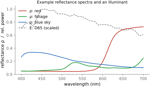
fig-bw-conversions
fig-bw-conversions · one colour photo → black & white several ways: single channel (R/G/B) · average · weighted luminance · red-filter channel mix (dark sky) · an isoluminant pair collapsing to one grey — the choices differ (Converting to B&W, Color technology)
• **how**: silicon photodiodes respond well into the **near-infrared**, so every camera ships with an **IR-cut filter** to keep IR from contaminating color. Two routes to NIR imaging: (1) **convert the camera** — remove the internal IR-cut filter (and optionally replace it with clear glass or an IR-pass filter); (2) **filter the lens** — an **IR-pass (visible-blocking) filter** (e.g. R72 / 720 nm) on a stock camera, at the cost of long exposures since most IR is being thrown away by the still-present internal cut filter.
• **what changes — the look**: **foliage glows bright white** (chlorophyll/leaf cell structure reflects NIR strongly) — the classic **"Wood effect"** (after R. W. Wood, 1910); **skin** goes smooth and waxy (NIR penetrates the surface, veins show); **blue sky darkens** and **haze is cut** (less Rayleigh scattering at longer wavelengths → see further); **water** goes inky black.
• **false-color IR**: since NIR is invisible, render it by **mapping bands to visible channels** (e.g. NIR→red, red→green, …) — the surreal magenta-foliage "Aerochrome" look; a channel-remapping choice, not a measurement.
• **uses beyond art**: **forensics & art conservation** (read faded ink, underdrawings, alterations beneath paint); **agriculture / remote sensing** — **NDVI** $=(\text{NIR}-\text{Red})/(\text{NIR}+\text{Red})$, the vegetation-health index that exploits the foliage-glows-in-NIR effect; **astronomy** (NIR pierces dust, redshifted light — e.g. JWST); and as an **extra channel** for computational photography (NIR-assisted denoising / dehazing / dark flash, cross-ref).