2.8 Noise, signal-to-noise ratio and dynamic range⧉
Noise earns a chapter of its own because, more than resolution or optics, noise is what ultimately limits our ability to measure and reconstruct an image. Almost everything else in this book (denoising, demosaicking, deblurring, HDR merging, depth from stereo, super-resolution) is at bottom an attempt to recover a clean signal from noisy measurements, and their performance is limited by how much noise corrupts the input. So understanding where noise comes from, how it scales with light, and which kind dominates when is not a side topic: it is the quiet constraint behind the whole field. It tells you what is recoverable and what is lost for good, how many photons or frames you need to reach a target quality, and, when a result disappoints, whether you are limited by your algorithm or by the physics of the measurement itself. Read this chapter as the floor under every later one.
2.8.1 Noise sources⧉
Counting photons is what makes a sensor linear, but counting is also where noise comes from. Take two photos of the same still scene at the same settings and they are not byte-for-byte identical; each pixel value jitters from frame to frame. Several physical sources contribute, and because they are statistically independent, their variances add, so to combine them we add variances ($\sigma^2$), not standard deviations (Figure 2.8.3).
Two numbers describe noise spread, and it pays to know why both exist. Variance (the mean squared deviation) is the quantity the mathematics wants: it is additive for independent sources — exactly what we just used, and the basis of the $1/\sqrt N$ averaging law in Denoising basics — it is the second moment that falls out of every Gaussian and least-squares derivation, and it composes cleanly under linear operations. But its units are squared (squared gray-levels, squared photons), so it means nothing to the eye. The standard deviation $\sigma$ (its square root) is the one people should read: it is back in the original units, directly comparable to the signal — the "$\sigma$" of error bars and the grain you actually see. Rule of thumb: derive and combine in variance, report in standard deviation.
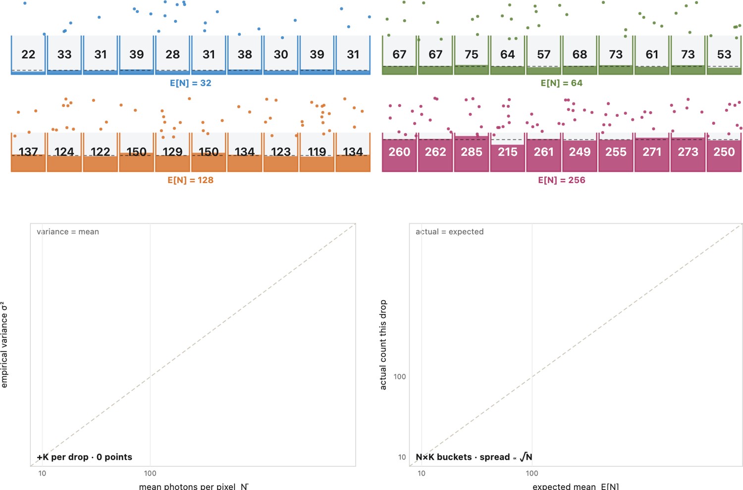
Photon (shot) noise is the deepest source, and it is not a defect of the sensor: it is the light itself. Light arrives as discrete photons at random times, so the count in a fixed interval fluctuates even from a perfectly steady source. The statistics are Poisson, and the defining property of a Poisson process is that its variance equals its mean (Hasinoff 2012 is the canonical short reference). So if a pixel collects $N$ photons on average, the variance of the count is $N$ and the standard deviation is
This is irreducible: no better sensor can remove it, because it is a property of light, not of electronics. It dominates the midtones and highlights, where $N$ is large. The only mitigation is averaging: average $N_f$ independent frames of the same scene and the shot noise drops by $\sqrt{N_f}$: the statistical basis of burst denoising and astrophotography stacking.
A Poisson process is the standard model for events that occur independently and at random, at a steady average rate, with no two at exactly the same instant: raindrops striking a tile, clicks of a Geiger counter, and, for us, photons landing on a pixel. It rests on three assumptions: the counts in non-overlapping intervals are independent; events arrive at a constant mean rate $\lambda$; and the process is memoryless (how long you have already waited says nothing about when the next event comes, so the gaps between events are exponentially distributed). Under these, the number of events in a fixed interval follows the Poisson distribution,
whose single parameter $\lambda$ is both its mean and its variance. That coincidence, $\text{variance} = \text{mean}$, is the whole of shot noise: catch $N$ photons on average and the count wobbles with standard deviation $\sqrt{N}$, so the noise grows as the square root of the signal and can never be zero. (Ideal laser light is exactly Poisson; thermal light bunches very slightly above it, but for photography Poisson is the right model.)
Even a flawless sensor is noisy, because light itself is grainy: photons arrive as discrete, randomly-timed events, so the count in any fixed interval follows Poisson statistics ($\sigma=\sqrt N$), and no electronics can remove it — the randomness is in the light, not the chip. The only true cure is collecting more photons: a bigger pixel, a wider aperture, a longer exposure, or averaging many frames. Crucially, raising ISO is not a cure — it is gain applied after capture, amplifying signal and shot noise together. This irreducible floor is why bigger sensors win, why shadows are noisy, and what every denoiser later in the book is ultimately fighting.
The remaining sources are added by the hardware:
- Read noise is added by the amplifier and the analog-to-digital converter (ADC) at readout. It is signal-independent (a roughly fixed amount regardless of brightness), so it dominates the shadows (where the signal is tiny) and sets the sensor's noise floor.
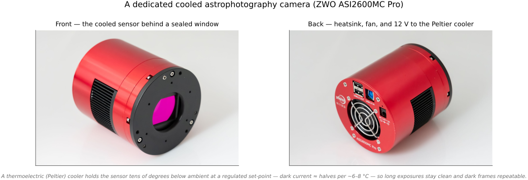
- Thermal (dark-current) noise comes from electrons freed by heat rather than light. It is independent of the scene but grows with exposure time and temperature, which is why long exposures and astrophotography call for sensor cooling and dark-frame subtraction (photographing the dark current with the shutter closed and subtracting it).
- Fixed-pattern noise is per-pixel non-uniformity: slightly different gain or offset at each photosite, plus hot or stuck pixels and banding. Because it is structured rather than random (the same pattern in every frame), it reads as worse than random noise of the same magnitude, and it is removed by calibration (flat and dark fields).
Sensor noise is a sum of distinct sources whose variances add, but each rules a different regime — so diagnosing a noisy image means asking which one you are seeing. Photon shot noise ($\propto\sqrt{\text{signal}}$) dominates the midtones and highlights, and any well-lit shot. Read noise is signal-independent and dominates the deep shadows and short exposures, setting the floor. Thermal / dark-current noise grows with exposure time and temperature — the long-exposure and astrophotography enemy. Quantization matters only with too few bits (L2.49). And fixed-pattern noise / PRNU — static per-pixel gain and offset variation — reads as a structured pattern and is removed by calibration (dark and flat fields). Match the symptom to the source before reaching for a fix.
The same five sources, as a reference table (what each varies with, where it dominates, and whether you can remove it):
| source | what it is | varies with | dominant regime | removable? |
|---|---|---|---|---|
| photon (shot) noise | Poisson statistics of photon arrival | $\sigma=\sqrt{N}$ — grows as √(signal) | midtones & highlights; every well-lit shot | no (fundamental — only more light helps) |
| read noise | amplifier + ADC at read-out | constant per read-out; relatively lower at higher analog ISO | deep shadows, short exposures (sets the floor) | no, but minimized; charge-binning pays it once |
| dark-current (thermal) | electrons freed by heat | exposure time × temperature (≈ doubles per ~6–8 °C) | long exposures, hot sensors, astro | partly — cooling + dark-frame subtraction |
| quantization | finite ADC bit depth | number of bits (negligible with enough) | only with too few bits / a heavy push | yes — more bits, dithering |
| fixed-pattern / PRNU | per-pixel gain & offset variation, hot pixels | static (same each frame); gain part scales with signal | structured pattern, visible in flats/darks | yes — flat- & dark-field calibration |
Dark current is the one noise source you can attack with a refrigerator. Because thermally-freed electrons roughly double for every ~6–8 °C, cooling the sensor a few tens of degrees below ambient cuts dark-current noise by a large factor, which is why dedicated astrophotography cameras bolt a thermoelectric (Peltier) cooler to the sensor and run it at a regulated set-point (say −10 °C or −20 °C). The set-point matters as much as the cooling: holding a fixed temperature makes the dark frames repeatable, so a library of master darks taken once can be subtracted from every light frame to remove both the dark-current pedestal and the hot pixels. Combined with the $1/\sqrt N$ stacking of many long sub-exposures (a later chapter), regulated cooling is what lets amateurs pull faint galaxies out of the noise over a night of integration (Figure 2.8.2).
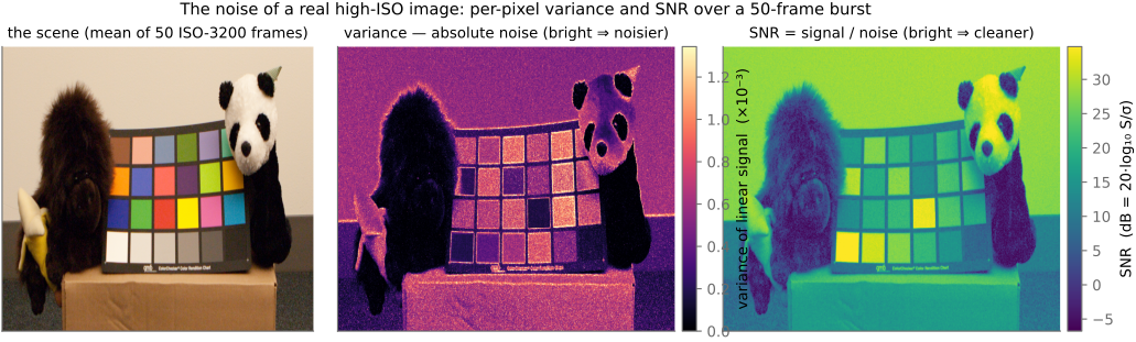
We can see that noise directly. Shoot a burst of one static scene at high ISO and take, for every pixel, its variance across the frames: the result is a map of the noise itself, laid over the picture (Figure 2.8.4). The noise is not uniform: it is heavier in the brighter regions (shot noise) and along edges, which is the clue to the rule that follows.
2.8.2 The algebra of noise⧉
Because the sources are independent, their variances add: the single most useful fact for reasoning about noise, and worth turning into a tool. For $N$ independent measurements each of variance $\sigma^2$, the sum has variance $N\sigma^2$ (standard deviation $\sqrt N\,\sigma$), while the average has variance $\sigma^2/N$ (standard deviation $\sigma/\sqrt N$). That $1/\sqrt N$ is the engine of all averaging-based denoising (a whole chapter later). The same algebra settles a subtler, very practical question: is it better to measure light with one big pixel, or with several small ones and add them up?
Take a patch that collects $N$ photons. Capture it with one big pixel: it counts $N$ photons (shot variance $N$, since Poisson variance $=$ mean) and adds the read noise once, $\sigma_r^2$. Now split the same patch into four small pixels, each catching $N/4$ photons. Summing their four readings recovers the signal $N$, and the shot noise is identical: the four shot variances $N/4$ add back to $N$, exactly the big pixel's. But each small pixel contributes its own read noise, so the sum carries $4\sigma_r^2$: the read noise is paid four times over. So, provided no light is lost in the gaps between photosites, the big pixel's only real advantage is read noise, not shot noise. Shot noise depends solely on how many photons you caught, never on how you diced up the sensor; read noise is charged once per read-out.
This is exactly why binning matters, and why how you bin matters. Charge binning (pooling the pixels' charge in the analog domain before it reaches the amplifier and ADC) reads the combined charge once, paying read noise a single time and recovering the full big-pixel advantage; this is the trick a good quad-Bayer sensor uses in low light. Digital binning (reading the four pixels separately and adding the numbers afterward) pays read noise four times and captures only the shot-noise equivalence. The gap is invisible in bright light (shot-noise-dominated) and decisive in the dark (read-noise-dominated). It also previews the affine model $\sigma^2 = g\,I + \sigma_r^2$ (developed shortly) from a new angle: aggregating $k$ measurements multiplies the read-noise term's contribution by $k$ unless you combine before read-out.
Add the readings of $k$ small pixels and you get the same Poisson (shot) noise as one big super-pixel that caught the same photons — but you pay the read noise $k$ times, once per read-out, instead of once. So the only fundamental advantage of a bigger pixel (or one longer exposure) over many smaller ones is the read noise, not the photon statistics — as long as no light is lost in the gaps. The same holds for aggregating along any dimension: summing $k$ short exposures, or $k$ burst frames, keeps the shot noise of the total light but charges read noise $k$ times. This is precisely why charge-domain binning (combine, then read once) beats digital summation (read $k$ times, then add) in the dark.
2.8.3 Signal-to-noise ratio: it's about ratios⧉
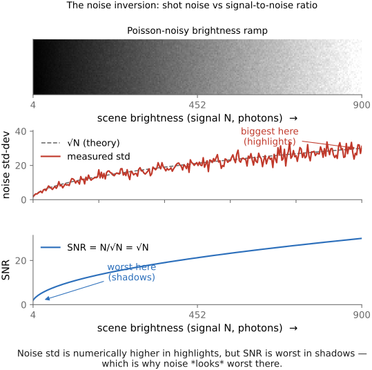
Here is the fact that surprises people and ties the whole part together. Since shot noise is $\sigma = \sqrt{N}$, the absolute noise is actually larger in the bright parts of the image than in the dark parts: a highlight collecting 10,000 photons has $\sigma = 100$, while a shadow collecting 100 photons has only $\sigma = 10$. And yet noise looks worst in the shadows. The resolution is that perception cares about the signal-to-noise ratio (SNR), not the absolute noise. For shot noise,
The SNR grows with brightness, so it is worst where the light is faintest (the shadows) even though the raw noise magnitude is smallest there (Figure 2.8.5). Ratios are all that matters. This is the same lesson that drives gamma/log encoding (we encode so that equal ratios get equal steps) and exactly why exposing to the right works: collecting more photons everywhere, especially in the shadows, raises $N$ and therefore raises the SNR where it is worst.
One caution before we go on, because the acronyms collide: SNR is not PSNR. The signal-to-noise ratio here is a property of a capture, the true signal at a pixel relative to the sensor's noise there ($\sqrt N$ for shot noise), and it answers how clean is this measurement? Peak signal-to-noise ratio (PSNR), which you meet whenever an algorithm is evaluated, is a different animal: a full-reference quality metric that compares a processed image $\hat I$ against a ground-truth reference $I$, computed from their mean-squared error as
where $\mathrm{peak}$ is the largest possible value (255 for 8-bit) and $\mathrm{MSE}=\tfrac1n\sum(\hat I-I)^2$. So SNR describes a photograph (how much noise a single measurement carries, with no reference needed), while PSNR scores a reconstruction against a known truth (how close a denoiser or codec got). They share "signal-to-noise" and a decibel scale and nothing else: one is a fact about the sensor, the other a yardstick for algorithms (and, as the metrics discussion later notes, a flawed one: because PSNR is just re-scaled MSE, it quietly rewards the blurry, safe answer).
Shot noise is Poisson, so its variance grows linearly with the signal ($\sigma^2 \propto N$) and its standard deviation grows only as the square root ($\sigma \propto \sqrt{N}$). Two consequences pull in opposite directions: the absolute noise is larger in highlights than in shadows (a 10,000-photon highlight has $\sigma=100$; a 100-photon shadow has $\sigma=10$), yet the SNR $= N/\sqrt{N} = \sqrt{N}$ is higher in the highlights — the signal outgrows the noise. So bright areas are noisier in absolute terms but cleaner to the eye; the shadows have the worst SNR (Figure 2.8.4, Figure 2.8.5). This is why exposing to the right and brighter scenes look smoother, and why we gamma/log-encode so equal ratios get equal steps.
The affine model, whose full story is the next section, settles a lot of everyday "will this help my noise?" questions at a glance. Read each move against $\sigma^2 = g\,I + \sigma_r^2$ (signal $I$, photon-gain slope $g$, read-noise floor $\sigma_r$), tracking what happens to the signal, the noise $\sigma$, and their ratio. The entries below are for the shot-noise-dominated regime (well-lit midtones); the read-noise term $\sigma_r$ changes only the two rows that mention it.
| scenario | signal | noise $\sigma$ | SNR | what is really going on |
|---|---|---|---|---|
| raise ISO by 1 stop (×2 analog gain) | ×2 | ×2 | ≈ same | amplifies signal and noise together and adds no photons. Read noise, applied after the gain, shrinks relative to the signal, so deep shadows come out a touch cleaner. Not a substitute for light. |
| brighten by 1 EV in software (×2) | ×2 | ×2 | unchanged | multiplies values already recorded, so it amplifies the noise baked in at capture. No shadow benefit, unlike raising ISO at capture. |
| darken by 1 EV in software (×½) | ×½ | ×½ | unchanged | pure scaling; the ratio is untouched (though it can still clip or quantize). |
| average $N$ frames | ×1 | ÷$\sqrt N$ | ×$\sqrt N$ | independent noise partly cancels while the signal stays: the $1/\sqrt N$ law behind burst denoising and stacking. |
| sum $N$ values | ×$N$ | ×$\sqrt N$ | ×$\sqrt N$ | variances add, so SNR grows just like averaging; but read noise is paid $N$ times if the values are read separately. |
| charge-bin $N$ pixels (combine, then read once) | ×$N$ | ×$\sqrt N$ | ×$\sqrt N$, cleaner shadows | same shot noise as a digital sum, but read noise is paid once, not $N$ times. Why quad-Bayer binning wins in low light. |
| gather 2× the light (wider aperture or longer exposure) | ×2 | ×$\sqrt 2$ | ×$\sqrt 2$ | the only move that collects more photons, so the only real, fundamental gain in SNR. Read noise unchanged. |
The pattern is stark: rescaling the numbers you already have (ISO, software exposure) never improves the signal-to-noise ratio; combining $N$ independent measurements improves it as $\sqrt N$; and the one thing that genuinely beats noise is collecting more light.
2.8.4 Noise variance is affine in pixel brightness⧉
Because the variances of these sources add, and because the dominant two scale so simply with the signal, the whole noise level follows a strikingly simple rule that we can measure directly from data.
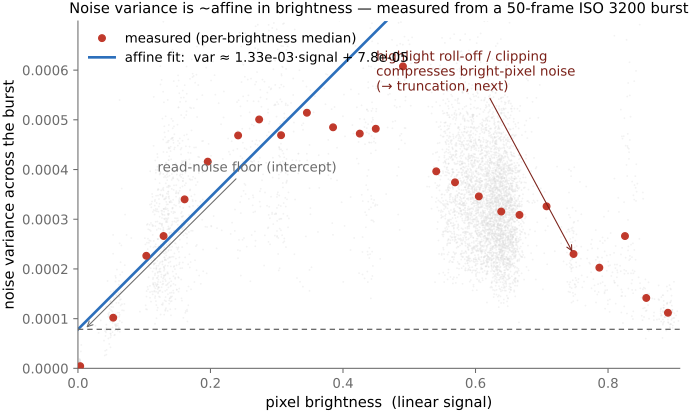
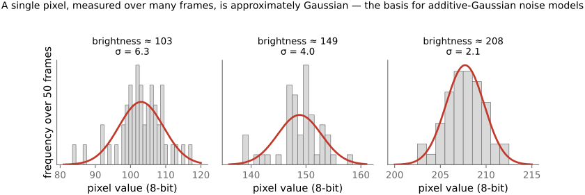
The variances add, and two terms dominate: shot noise contributes an amount proportional to the signal (Poisson, variance = mean, scaled by the gain) and read noise a constant floor. So the total is variance ≈ gain·signal + read² — a straight line in brightness (Figure 2.8.6). The slope is the photon gain (it steepens with ISO, which amplifies the signal and its shot noise together); the intercept is the read-noise floor. We can measure it without any model: take an aligned burst of a static scene and, per pixel, plot the variance across frames against the mean. And a single pixel's value over many frames is ≈ Gaussian (Figure 2.8.7) — which is what licenses modeling per-pixel noise as additive Gaussian.
Read the affine model the other way and it becomes a noise simulator: the quickest way to turn a clean image into realistic noisy data, for stress-testing a denoiser or building the synthetic training pairs this book leans on (Deep learning). Two rules make or break it. First, work on a linear image, never a gamma-encoded one: variance is affine in brightness only in linear light, so noise added after the tone curve injects the wrong amount in the shadows, exactly where it shows, and looks plainly fake. Second, and less often stated, do the physics in the sensor's native currency, electrons (photon counts), because that is the only unit in which shot noise is exactly Poisson. So convert the linear image to a mean electron count, draw the shot term as a Poisson variate and the read term as a Gaussian, then carry the result back out through gain, black level, clipping, and quantization (Algorithm 2.8.1):
for each linear pixel value I in [0, 1]:      # 1.0 == a full photosite well; NOT gamma-encoded
    N_e   = I * full_well                     # to ELECTRONS: the photon scale
    shot  = poisson(mean = N_e)               # shot noise IS a Poisson count  (var = mean, sigma = sqrt(N))
    e     = shot + gaussian(0, read_noise_e)  # read/constant noise: zero-mean Gaussian, in electrons
    DN    = round(e * gain + black_level)      # to code values: gain folds in ISO; add the pedestal
    DN    = clamp(DN, 0, max_DN)              # clip: highlights at full well, floor at 0
    I_out = (DN - black_level) / (max_DN - black_level)   # back to linear [0, 1]
# apply gamma / the display curve only AFTER this loop, never before
The units are the whole game. Three currencies coexist and it pays to keep them straight. The scene-linear image is normalized, values in $[0,1]$ with $1.0$ standing for a full well. The sensor counts in electrons (photons converted at the quantum efficiency $\eta$), and this is where shot noise lives: a mean of $N$ electrons gives a Poisson count whose variance is $N$, so $\sigma=\sqrt N$. The ADC finally reports digital numbers (DN, or ADU: the raw code values), related to electrons by a gain $g$ in DN per electron, into which the ISO setting folds. The one non-negotiable step is the conversion $N=I\cdot N_{\text{full}}$ before the Poisson draw: "variance equals mean" holds only for the count, so drawing Poisson in normalized $[0,1]$ or in DN gets the noise magnitude wrong by whatever the scale factor is. Multiply the clean image up into electrons, add the noise there, and only then scale back. Typical numbers: a full-frame photosite holds $N_{\text{full}}\approx30{,}000$-$60{,}000$ electrons, a phone pixel a few thousand; read noise $\sigma_r$ is $\sim1$-$3\,e^-$ on good CMOS and rises with ISO.
In electrons the linear (shot) term is not a fitted constant, it is pure physics. Write the normalized linear measurement as $x\in[0,1]$, a fraction of full well. The mean electron count is
with $N_{\text{full}}$ the full-well capacity, the electrons a photosite holds at saturation. Shot noise is Poisson, so its variance in electrons equals that mean:
That is the whole "linear term $a\,x$": a straight line through the origin whose slope is simply the well capacity, with nothing to tune. And the slope is set entirely by physics, by how many photons the exposure delivers and the quantum efficiency $\eta$ that converts them to electrons ($N=\eta\,N_{\text{photons}}$, so $N_{\text{full}}=\eta\,N_{\text{photons at saturation}}$). The normalized slope $a$ of L2.44 looks like a fitted number only because of the change of units: rescaling those electrons back into $[0,1]$ (divide by $N_{\text{full}}$) or into DN (multiply by the gain) turns the clean $N_{\text{full}}\,x$ into $a\,x$. In electrons it is just the photon count.
The affine Gaussian of L2.44 is simply the fast approximation to this recipe: it swaps the Poisson draw for a Gaussian of the same variance and folds the two conversions into two constants, giving $\sigma^2 = a\,I + b$ with $a$ the photon slope (gain times full-well) and $b$ the read-noise floor, both in normalized units. Those constants span a wide range with sensor size and ISO (values for $I$ in $[0,1]$): a large full-frame sensor runs from about $a\approx10^{-5},\ b\approx10^{-9}$ at base ISO to $a\approx10^{-3},\ b\approx10^{-7}$ pushed high; a small phone sensor from about $a\approx10^{-4},\ b\approx10^{-8}$ at base ISO to $a\approx10^{-2},\ b\approx10^{-6}$ high. Smaller wells and more amplification both steepen $a$ and lift $b$.
When is that Gaussian good enough, and when does it break? A Poisson count is a sum of many independent tiny arrivals, so by the central limit theorem it approaches a Gaussian of the same mean and variance as the count grows: $\text{Poisson}(N)\approx\mathcal N(N,\,N)$. Its skewness is $1/\sqrt N$, so the bell is nearly symmetric once $N$ is a few dozen, and in midtones and highlights (thousands of electrons) the Gaussian is indistinguishable from the truth and cheaper to draw. It breaks in exactly the place that matters, the deep shadows, where $N$ falls to single digits. Three things go wrong at low counts: the distribution is discrete (you caught 3 photons or 4, never 3.5), it is right-skewed (a tail toward more photons, none toward fewer), and it is non-negative, whereas a Gaussian will hand back negative electron counts, which are unphysical and, once clipped at zero, bias the shadows bright (the truncation of L2.45 below). Rule of thumb: use the true Poisson draw below a couple of dozen electrons and the Gaussian above; a simulator that wants faithful shadows, or that models the low-light or photon-counting regime at all, must use Poisson. The same crossover is a free speed win, since a Poisson sampler is slow for large means while a Gaussian is not, so switching near $N\approx20$ costs no accuracy and speeds up the bright pixels.
Drawing Poisson noise. In Python, NumPy does it vectorized over the whole image at once, each pixel drawn at its own mean:
import numpy as np
rng = np.random.default_rng()
electrons = rng.poisson(mean_e)   # mean_e: float array of electron counts -> integer counts
In C++, the standard library provides it in <random>; the mean is a construction parameter, so a per-pixel mean means constructing (or re-parameterizing) the distribution for each pixel:
#include <random>
std::mt19937_64 rng(seed);
std::poisson_distribution<long long> shot(mean_e);  // mean_e > 0
long long k = shot(rng);                            // one Poisson electron count
Put together, the whole simulator is short. In Python (NumPy, whole image at once) (Listing 2.8.1):
import numpy as np

def add_sensor_noise(img, full_well=30000.0, read_noise_e=2.0,
                     bit_depth=14, black_level_dn=0.0, rng=None):
    """Physically-based sensor noise on a scene-LINEAR image where 1.0 == full well.

    Everything happens in electrons, the only unit in which shot noise is Poisson.
    Returns a linear float image back in [0, 1] with the noise baked in.
    """
    rng = np.random.default_rng() if rng is None else rng
    max_dn = float((1 << bit_depth) - 1)
    gain   = (max_dn - black_level_dn) / full_well          # DN per electron

    mean_e    = np.clip(img, 0.0, None) * full_well         # 1. to electrons
    electrons = rng.poisson(mean_e).astype(np.float64)      # 2. shot: Poisson count
    electrons += rng.normal(0.0, read_noise_e, img.shape)   # 3. read: Gaussian, in electrons

    dn = np.round(electrons * gain + black_level_dn)        # 4. to DN: gain + pedestal
    dn = np.clip(dn, 0.0, max_dn)                           #    clip to the ADC range
    return (dn - black_level_dn) / (max_dn - black_level_dn)  # 5. back to linear [0, 1]
and the same in C++ (per pixel, standard library only) (Listing 2.8.2):
#include <random>
#include <vector>
#include <cstdint>
#include <cmath>
#include <algorithm>

// Physically-based sensor noise on a scene-LINEAR image where 1.0 == full well.
// Everything happens in electrons, the only unit in which shot noise is Poisson.
// `img` is row-major linear pixels in [0,1]; modified in place, back in [0,1].
void add_sensor_noise(std::vector<float>& img,
                      double        full_well      = 30000.0,
                      double        read_noise_e   = 2.0,
                      int           bit_depth      = 14,
                      double        black_level_dn = 0.0,
                      std::uint64_t seed           = 0)
{
    std::mt19937_64 rng(seed);
    std::normal_distribution<double> read(0.0, read_noise_e);
    const double max_dn = double((1u << bit_depth) - 1u);
    const double gain   = (max_dn - black_level_dn) / full_well;   // DN per electron

    for (float& px : img) {
        double mean_e = std::max(0.0, double(px)) * full_well;     // 1. to electrons
        double e;
        if (mean_e > 0.0) {                                        // 2. shot: Poisson count
            std::poisson_distribution<long long> shot(mean_e);    //    (mean must be > 0)
            e = double(shot(rng));
        } else {
            e = 0.0;
        }
        e += read(rng);                                           // 3. read: Gaussian, in electrons
        double dn = std::round(e * gain + black_level_dn);        // 4. to DN: gain + pedestal
        dn = std::min(max_dn, std::max(0.0, dn));                 //    clip to the ADC range
        px = float((dn - black_level_dn) / (max_dn - black_level_dn)); // 5. back to [0, 1]
    }
}
The cardinal mistake is the one-liner everyone reaches for first: a single constant-$\sigma$ Gaussian added to a gamma-encoded image. It is signal-independent (no shot noise) and in the wrong space, so it looks wrong in exactly the shadows where noise matters. Real noise is Poisson plus Gaussian, in linear electrons; everything else is a shortcut.
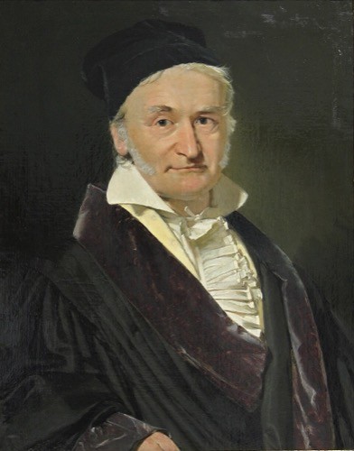 Carl Friedrich Gauss (1777–1855), the "prince of mathematicians," appears repeatedly in this book, and you have just met him in the bell curve. The Gaussian (normal) distribution that a noisy pixel traces over many frames is his, and so is least squares, which he used in 1801 to recover the orbit of the dwarf planet Ceres from a handful of sightings and which underlies nearly every fit and reconstruction we do. The same name returns as the Gaussian blur, Gaussian elimination inside our linear solvers, and the Gauss–Seidel iteration. That a sum of many small independent effects collapses into one bell shape (the central limit theorem) is exactly why the additive-Gaussian noise model keeps working. Portrait: painting by Christian Albrecht Jensen, 1840, public domain (via Wikimedia Commons).
The affine model and the Gaussian shape are the ideal. Real recorded values break the ideal in one important way at the extremes.
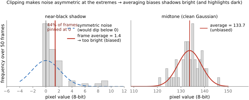
A recorded value is clamped to $[0,\text{max}]$. Near black the negative half of the noise is cut off and frames pile up at 0; near white the positive half is. So at the extremes the noise distribution is asymmetric, with its mean pushed inward (Figure 2.8.8). The consequence for denoising: a naive average or smoothing returns that biased mean, so it makes shadows come out too bright and highlights too dark — a bias every denoiser must correct for (we return to it in Denoising, BASIC).
That clipping caveat is the first crack in the affine model, and a larger one is worth planting now. The law $\sigma^2 \approx a\,I + b$ describes the noise as the sensor hands it over (the raw mosaic, straight off the ADC); it is a fact about the sensor, not about the final photograph. Run that raw through the computational-photography pipeline and the clean affine line bends. A burst merge (align-and-average $N$ frames, Denoising basics) drives the variance toward $1/N$ of a single frame, but unevenly (the robust merge keeps more frames in still regions than near moving edges), so the noise becomes spatially varying, and highlight clipping means it is no longer even affine in brightness. Demosaicking (Demosaicking) bends it too: an interpolated color is a weighted average of neighboring pixels, and averaging shrinks variance, so reconstructed pixels are quieter than the ones actually measured, by different amounts, pixel to pixel. After a few ISP stages the tidy 'gain·signal + read²' line is gone, and a downstream algorithm that still assumes it (a plain AWGN denoiser, say) is fitting a model the data no longer obeys.
Manufacturers know this and design around it: many sensors deliberately lift the black point before digitizing. They add a fixed offset (a "black level" or bias, a few hundred code values) to the signal, so the whole bell of the read noise, negative excursions included, lands above zero and is recorded rather than clipped (Canon, for instance, sits its black level around code 512 or 2048 on 14-bit raw; other makers similar). The raw file then carries an explicit black-level tag that the converter subtracts back out. Keeping the noise unclipped this way is exactly what lets noise-weighted averaging, flat/dark calibration, and shadow-lifting stay unbiased down in the darkest tones, at the cost of a sliver of headroom. One discipline follows: after subtracting the black level, near-black pixels can legitimately go slightly negative, and that must be preserved, not clamped, all the way until display, or the bias creeps right back in.
The affine model is also a recipe: it is how you turn a clean image into realistic noisy data: for testing a denoiser, or for the synthetic training pairs this book leans on (→ synthetic data in Deep learning). Work in linear light, think in electrons, and apply the sources in capture order:
- Scale to electrons. Map the clean linear image to a photon count, $N = I\cdot N_{\text{full}}$, or pick an exposure level; fewer electrons means a noisier result. This chooses where on the SNR curve you land.
- Shot noise. Replace each pixel by a Poisson draw with mean $N$ (
numpy.random.poisson(N)), or a Gaussian of variance $N$ when $N$ is large. This is the $\sigma=\sqrt N$ floor: it is signal-dependent, drawn per pixel, not added as a constant. - Read noise. Add zero-mean Gaussian noise of standard deviation $\sigma_r$ electrons (the floor; larger at higher ISO).
- Gain, black level, clip, quantize. Multiply by the analog/ISO gain, add the black-level offset, clip at full-well (highlights), and quantize to the bit depth.
- Re-encode. Apply gamma / the camera curve last, so the noise you built in linear light decodes correctly.
The cardinal mistake is adding a single constant-σ Gaussian to a gamma-encoded image: that is neither signal-dependent (no shot noise) nor in the right space, and it looks wrong in exactly the shadows where it matters. Real noise is Poisson + Gaussian, in linear electrons; everything else is a shortcut.
2.8.5 Noise as a function of ISO⧉
The affine constants $a$ and $b$ are not fixed properties of a sensor: they slide with the ISO setting, because ISO is an analog gain applied partway down the readout chain, and it matters a great deal where each noise source enters relative to that amplifier. Three sources, three positions:
- Photon (shot) noise enters at capture, in electrons, with variance equal to the mean count $N=x\,N_{\text{full}}$. It is then amplified along with the signal.
- Pre-gain read noise $\sigma_{\text{pre}}$ (electrons) is the noise of the photosite and the first source-follower, injected before the analog gain, so it is amplified exactly like the signal.
- Post-gain read noise $\sigma_{\text{post}}$ is everything added after amplification: the analog-to-digital converter and the downstream electronics. The gain never touches it.
Write the analog gain as $g$ (in DN per electron), rising with ISO. The mean recorded value is $\mu = g\,N$ (DN), and the three variances add, each in the domain it lives in. Referred to the output (DN$^2$):
This is the same affine line $\sigma^2 = a\,\mu + b$, now with its constants named by physics: the slope $a=g$ is the gain, so it rises in direct proportion to ISO, and the intercept $b = g^2\,\sigma_{\text{pre}}^2 + \sigma_{\text{post}}^2$ is the read-noise floor, a sum of a term the gain amplifies and a term it does not. (The photon term reads $g\,\mu$ because in electrons its variance is $N=\mu/g$, amplified by $g^2$.)
The revealing move is to refer that floor back to the input, dividing by $g^2$ to read it in electrons:
As ISO climbs, the post-gain term shrinks as $1/g^2$ and the input-referred read noise falls toward the floor $\sigma_{\text{pre}}$. That single curve, read noise in electrons versus ISO, is the whole story of a sensor's low-light behavior (Figure 2.8.9).
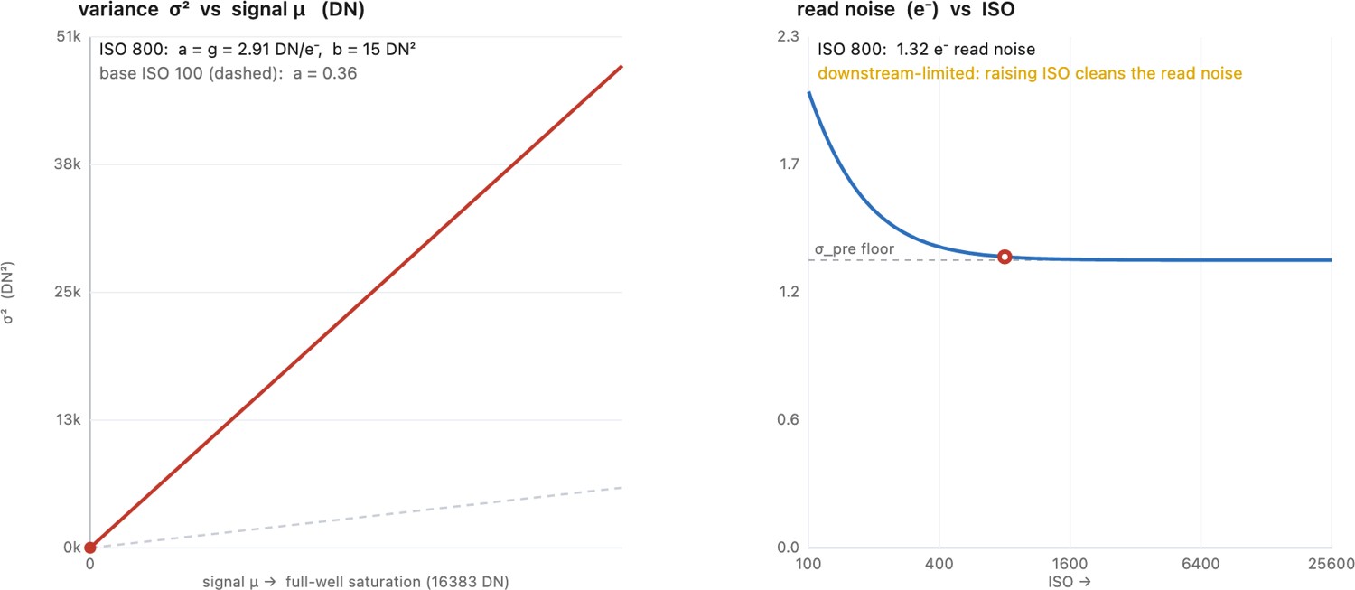
The two constants that do not depend on ISO are the pre- and post-amplification read noises; tabulating them (with the full well) fixes $a(g)$ and $b(g)$ at every ISO. Representative figures for a few sensor classes (order-of-magnitude, for illustration; Bill Claff's measured read-noise curves at photonstophotos.net are the reference):
| Sensor (example) | full well $N_{\text{full}}$ (e⁻) | pre-gain $\sigma_{\text{pre}}$ (e⁻) | post-gain $\sigma_{\text{post}}$ (e⁻, base ISO) | dual-gain step | character |
|---|---|---|---|---|---|
| Modern BSI full-frame (Sony α7 IV, Nikon Z6 II) | ~45,000 | ~1.2 | ~1.5 | ~ISO 500 | ISO-invariant above the step |
| Low-light-tuned DCG (Sony α7S III) | ~28,000 | ~1.0 | ~1.3 | ~ISO 640 | strongly ISO-invariant |
| Modern Canon (EOS R5 / R6) | ~50,000 | ~1.3 | ~2 | ~ISO 400 | mostly ISO-invariant |
| Older CMOS, off-chip ADC (Canon 5D Mark III, 2012) | ~68,000 | ~2.5 | ~35 | none | downstream-limited: raising ISO genuinely helps |
| Small pixel / phone (quad-Bayer) | ~6,000 | ~1.5 | ~2 | ~ISO 500 | binning + DCG in the dark |
What modern sensors do about it: ISO invariance and dual conversion gain. Two facts fall straight out of the input-referred equation. First, ISO invariance. If the pre-gain noise already dominates the floor at low ISO ($g^2\sigma_{\text{pre}}^2 \gg \sigma_{\text{post}}^2$), then $\sigma_{\text{read}}\approx\sigma_{\text{pre}}$ at every ISO, and raising ISO in the camera buys nothing that brightening the raw file in software could not. Such a sensor is called ISO-invariant: you may as well shoot at base ISO to protect the highlights and lift the shadows in post, with no noise penalty. This is where nearly every mirrorless sensor since about 2016 lives, because on-chip column ADCs have driven $\sigma_{\text{post}}$ almost to nothing. The older arrangement, an off-chip ADC with large downstream noise (many DSLRs into the early 2010s), sat at the opposite extreme: $\sigma_{\text{post}}$ dominated at low ISO, so cranking the analog gain genuinely lowered the input-referred read noise, and "expose at the ISO you actually need" was real advice, not superstition. In affine-model terms, ISO invariance is just the statement that the input-referred intercept $b/g^2$ is already flat.
Second, dual conversion gain. A photosite cannot at once hold a huge charge (for highlight headroom in bright light) and convert that charge to voltage with tiny noise (for clean shadows in the dark); the conversion gain that trades between them is a hardware setting. Modern sensors refuse to choose and build two readout modes: a low-conversion-gain mode with a large full well and higher read noise for bright scenes, and a high-conversion-gain mode with a smaller well but markedly lower $\sigma_{\text{pre}}$ that switches in above a threshold ISO. On a read-noise-versus-ISO plot this appears as a sudden step down at that ISO (the drop near ISO 500-800 on many bodies), where a higher ISO is actually cleaner than a slightly lower one. In our model the switch changes the physical constants themselves: at the threshold both $N_{\text{full}}$ and $\sigma_{\text{pre}}$ drop, so both the slope $a$ and the floor $b$ jump. The affine model is then not one line across all ISOs but a family of lines with a break at the dual-gain point.
The upshot ties the section together: $a$ and $b$ are not sensor constants but functions of ISO, with $a\propto g$ and $b=g^2\sigma_{\text{pre}}^2+\sigma_{\text{post}}^2$; ISO invariance is the regime where the input-referred floor $b/g^2$ is flat; and dual gain is a deliberate step in $\sigma_{\text{pre}}$ (and full well) that resets both constants at a chosen ISO. A denoiser or raw pipeline handed the wrong $a,b$ for the ISO, or blind to the dual-gain break, mis-models the noise in exactly the shadows it is trying to protect.
2.8.6 Dynamic range⧉
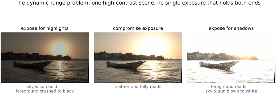
Two extremes bound what a single exposure can hold. At the top, a pixel's well saturates: once it has counted its full-well capacity of electrons, more light adds nothing and the highlight clips to white. At the bottom, the read-noise floor sets the dimmest signal still distinguishable from noise. The ratio of the two is the sensor's dynamic range: how much of a high-contrast scene a single exposure can capture. When a scene's range exceeds the sensor's (a bright window and a dim interior in one frame), no single exposure holds both ends, which is the motivation for high-dynamic-range (HDR) imaging, merging several exposures (Multiple-exposure part) (Figure 2.8.10). Like everything else a photographer counts, dynamic range is quoted in stops (factors of two), which connects it straight to the exposure controls.
There is one more limit that no sensor spec sheet lists: the lens. Bright parts of a scene scatter stray light inside the lens and camera body (faint reflections off every element surface, the diaphragm blades, and the barrel walls) that settle as a veil of light spread across the whole frame. This veiling glare, the diffuse cousin of lens flare, lifts the darkest tones off true black, raising the effective noise floor from the optical side just as read noise raises it from the electronic side. It therefore caps the dynamic range a real photograph can reach below whatever the bare sensor could deliver, and it bites hardest exactly when dynamic range matters most, shooting a dim subject against a bright source. It is why lens coatings, hoods, and a clean front element buy real shadow contrast, and why the deepest blacks in a studio shot are easier to protect than those in a backlit scene. Flare and veiling glare get their full treatment as optical defects in Aberrations and optical challenges (§10.1).
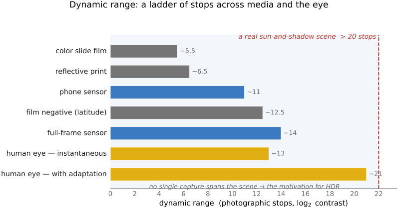
How wide a range, exactly? It helps to put numbers on it, because the dynamic ranges of real media and of the eye differ by a lot (Figure 2.8.11). A color slide is narrow, only about 5–6 stops; a reflective print about 6–7; a film negative is famously forgiving at roughly 12–13 stops of latitude; a phone sensor manages about 10–12 and a full-frame sensor about 14. The human eye sees about 10–14 stops instantaneously, but allow it to adapt (the slow re-centering of the retinal response covered with perception) and it spans 20+ stops over time; some animals do better still within their niche. Against all of these, an outdoor sun-and-shadow scene can exceed 20 stops in a single frame, which is precisely why no single capture holds it, and why HDR exists.
Recovering an underexposed shot: full-frame vs. phone. The clearest way to feel that dynamic range scales with photosite size is to break one. Shoot the same underexposed scene as raw on a full-frame camera and on a phone, then push the exposure up in software by three or four stops (Figure 2.8.12). The full-frame frame cleans up (its deep full-well and low read-noise floor give it the headroom to be lifted) while the phone frame breaks into shadow noise and banding, because lifting the exposure also amplifies its read-noise floor, which sat much closer to the signal to begin with. That is a direct, visible demonstration that dynamic range scales with photosite (and sensor) size, and exactly why phones lean on burst capture and HDR+ (Multiple-exposure part) rather than trusting a single exposure. It is also a coding exercise: see Exercises & Experiments.
A single exposure records from a top — the photosite's full-well capacity, where it saturates and clips to white — down to a bottom — the noise floor, the read noise that drowns the shadows. Their ratio is the dynamic range, quoted in stops. You widen it with a bigger well (larger photosites — why a full-frame sensor out-ranges a phone) or a lower floor (cooling, lower read noise), and you beat it altogether by merging multiple exposures (HDR). This is the capture-side companion to the quantization lesson below: what bounds a single shot is this range — full-well over floor — not the number of bits.
This is also the right moment to deflate a worry beginners often have about digital capture: that the image is quantized into a finite number of levels, and that this stair-stepping is what limits quality. It almost never is.
With enough bits and a sane encoding, what limits image quality is noise and dynamic range — the two quantities of this section — not the number of levels the analog-to-digital converter (ADC) offers. The noise floor and the full well bound what you can record; the quantization step, once it sits below the noise, is invisible. (Indeed, a little noise dithers the quantization, hiding it further.) The one place levels do bite is banding in the deep shadows of a linearly-encoded image — too few codes where the eye, working in ratios, is most sensitive — and that is exactly the problem gamma encoding exists to solve, by spending code levels perceptually (Measuring and encoding color). So "rarely" is not "never." We meet this lesson again in BASIC → Image representation → Float vs 8-bit, where floats with headroom are the sane default.
These three facts (that noise is the jitter of a photon count, that the signal-to-noise ratio is worst in the shadows, and that dynamic range is the full-well-over-floor a single exposure can hold) recur on nearly every later page: in how a photographer exposes to the right, in high-dynamic-range merging (Multiple-exposure part), and in the denoising of the basic pipeline. With measurement and its limits now in hand, the part turns next to what a second viewpoint buys you (depth), and then to the eye that will finally judge the result.
2.8.7 Regimes, and how close we are to the limits⧉
Pulling the chapter together: which noise matters depends entirely on how much light you have, and a single picture usually spans several regimes at once.
- Bright light / highlights — shot-noise-limited. Plenty of photons, so shot noise ($\sqrt N$) dominates and read noise is negligible. SNR is excellent and only improves with more light; nothing but more photons (or a bigger sensor) helps.
- Deep shadows / low light — read-noise-limited. Few photons, so the constant read-noise floor dominates and sets where the image dissolves into mush. This is where sensor engineering still moves the needle and where computational averaging (bursts) buys real ground.
- Long exposures / heat — dark-current-limited. Time and temperature let thermal electrons pile up; cooling and dark-frame subtraction are the cure.
The same three regimes bound dynamic range, which is just full-well capacity ÷ read-noise floor (L2.48): the top set by how many electrons a pixel holds before clipping, the bottom by the read noise.
How close are we to the theoretical limits? On two of the three axes, modern sensors are already close to their physical limits.
- Quantum efficiency, the fraction of arriving photons actually converted to electrons, is already around 80–95 % in good back-illuminated sensors, so there is at most a few tenths of a stop of light-gathering left to win. In bright light we are essentially at the shot-noise limit: a perfect sensor would be only marginally cleaner, because the noise is in the light itself (L2.42).
- Read noise has fallen to ~1–2 electrons on the best CMOS, and specialized scientific CMOS and electron-multiplying sensors reach sub-electron read noise, within sight of counting individual photons (the single-photon avalanche diodes of the Advanced part do exactly that).
- Full-well capacity, and hence single-exposure dynamic range, is the axis still bound by pixel area and electrostatics, and it is precisely the one that has plateaued (the previous chapter's curves): a pixel of a given size can only hold so many electrons before it saturates.
So the photons themselves are nearly free and nearly all counted; what stays scarce is holding and reading them without adding noise, and there physics has almost run out of room. That is exactly why the frontier moved off the single capture and onto multi-frame computation (averaging down the floor and merging exposures to beat the well), the bridge from this chapter's physics to the rest of the book.
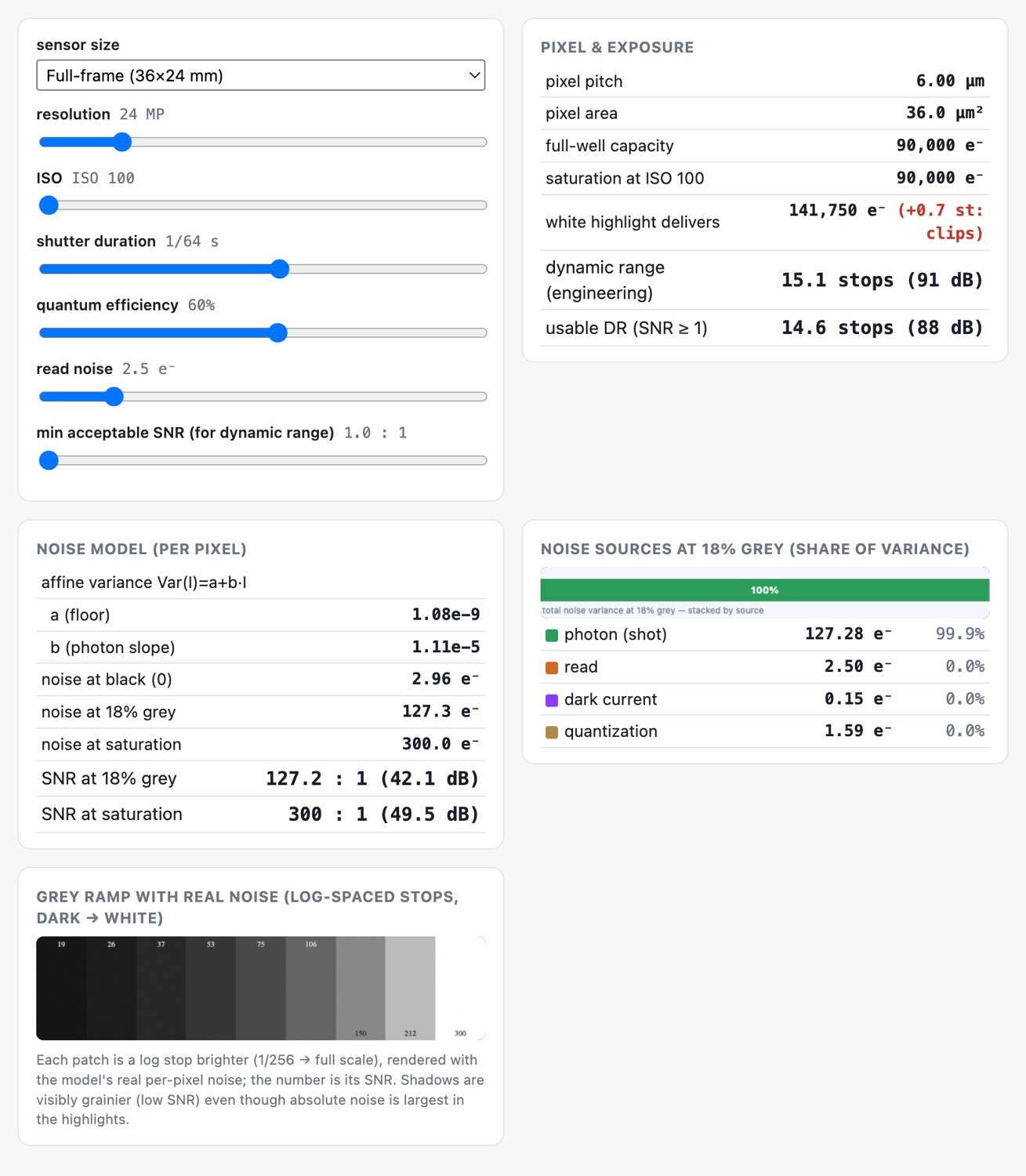
The whole budget is easiest to feel by turning the dials yourself (Figure 2.8.13).
Recap: big lessons of this chapter
Two numbers describe noise spread, and it pays to know why both exist. Variance (the mean squared deviation) is the quantity the mathematics wants: it is additive for independent sources — exactly what we just used, and the basis of the $1/\sqrt N$ averaging law in Denoising basics — it is the second moment that falls out of every Gaussian and least-squares derivation, and it composes cleanly under linear operations. But its units are squared (squared gray-levels, squared photons), so it means nothing to the eye. The standard deviation $\sigma$ (its square root) is the one people should read: it is back in the original units, directly comparable to the signal — the "$\sigma$" of error bars and the grain you actually see. Rule of thumb: derive and combine in variance, report in standard deviation.
Even a flawless sensor is noisy, because light itself is grainy: photons arrive as discrete, randomly-timed events, so the count in any fixed interval follows Poisson statistics ($\sigma=\sqrt N$), and no electronics can remove it — the randomness is in the light, not the chip. The only true cure is collecting more photons: a bigger pixel, a wider aperture, a longer exposure, or averaging many frames. Crucially, raising ISO is not a cure — it is gain applied after capture, amplifying signal and shot noise together. This irreducible floor is why bigger sensors win, why shadows are noisy, and what every denoiser later in the book is ultimately fighting.
Sensor noise is a sum of distinct sources whose variances add, but each rules a different regime — so diagnosing a noisy image means asking which one you are seeing. Photon shot noise ($\propto\sqrt{\text{signal}}$) dominates the midtones and highlights, and any well-lit shot. Read noise is signal-independent and dominates the deep shadows and short exposures, setting the floor. Thermal / dark-current noise grows with exposure time and temperature — the long-exposure and astrophotography enemy. Quantization matters only with too few bits (L2.49). And fixed-pattern noise / PRNU — static per-pixel gain and offset variation — reads as a structured pattern and is removed by calibration (dark and flat fields). Match the symptom to the source before reaching for a fix.
Add the readings of $k$ small pixels and you get the same Poisson (shot) noise as one big super-pixel that caught the same photons — but you pay the read noise $k$ times, once per read-out, instead of once. So the only fundamental advantage of a bigger pixel (or one longer exposure) over many smaller ones is the read noise, not the photon statistics — as long as no light is lost in the gaps. The same holds for aggregating along any dimension: summing $k$ short exposures, or $k$ burst frames, keeps the shot noise of the total light but charges read noise $k$ times. This is precisely why charge-domain binning (combine, then read once) beats digital summation (read $k$ times, then add) in the dark.
Shot noise is Poisson, so its variance grows linearly with the signal ($\sigma^2 \propto N$) and its standard deviation grows only as the square root ($\sigma \propto \sqrt{N}$). Two consequences pull in opposite directions: the absolute noise is larger in highlights than in shadows (a 10,000-photon highlight has $\sigma=100$; a 100-photon shadow has $\sigma=10$), yet the SNR $= N/\sqrt{N} = \sqrt{N}$ is higher in the highlights — the signal outgrows the noise. So bright areas are noisier in absolute terms but cleaner to the eye; the shadows have the worst SNR (Figure 2.8.4, Figure 2.8.5). This is why exposing to the right and brighter scenes look smoother, and why we gamma/log-encode so equal ratios get equal steps.
The variances add, and two terms dominate: shot noise contributes an amount proportional to the signal (Poisson, variance = mean, scaled by the gain) and read noise a constant floor. So the total is variance ≈ gain·signal + read² — a straight line in brightness (Figure 2.8.6). The slope is the photon gain (it steepens with ISO, which amplifies the signal and its shot noise together); the intercept is the read-noise floor. We can measure it without any model: take an aligned burst of a static scene and, per pixel, plot the variance across frames against the mean. And a single pixel's value over many frames is ≈ Gaussian (Figure 2.8.7) — which is what licenses modeling per-pixel noise as additive Gaussian.
A recorded value is clamped to $[0,\text{max}]$. Near black the negative half of the noise is cut off and frames pile up at 0; near white the positive half is. So at the extremes the noise distribution is asymmetric, with its mean pushed inward (Figure 2.8.8). The consequence for denoising: a naive average or smoothing returns that biased mean, so it makes shadows come out too bright and highlights too dark — a bias every denoiser must correct for (we return to it in Denoising, BASIC).
A single exposure records from a top — the photosite's full-well capacity, where it saturates and clips to white — down to a bottom — the noise floor, the read noise that drowns the shadows. Their ratio is the dynamic range, quoted in stops. You widen it with a bigger well (larger photosites — why a full-frame sensor out-ranges a phone) or a lower floor (cooling, lower read noise), and you beat it altogether by merging multiple exposures (HDR). This is the capture-side companion to the quantization lesson below: what bounds a single shot is this range — full-well over floor — not the number of bits.
With enough bits and a sane encoding, what limits image quality is noise and dynamic range — the two quantities of this section — not the number of levels the analog-to-digital converter (ADC) offers. The noise floor and the full well bound what you can record; the quantization step, once it sits below the noise, is invisible. (Indeed, a little noise dithers the quantization, hiding it further.) The one place levels do bite is banding in the deep shadows of a linearly-encoded image — too few codes where the eye, working in ratios, is most sensitive — and that is exactly the problem gamma encoding exists to solve, by spending code levels perceptually (Measuring and encoding color). So "rarely" is not "never." We meet this lesson again in BASIC → Image representation → Float vs 8-bit, where floats with headroom are the sane default.