3.4 Sensing color: multiplexing strategies⧉
A bare image sensor is usually color-blind (each photosite counts photons regardless of wavelength), so to capture color we must somehow take three (or more) measurements where a given photosite provides only one. Every color camera multiplexes those measurements across some axis, and there are several ways to do it, each spending a different axis (Figure 3.4.1).
Strip away the color filter and a sensor is monochrome at the pixel: each photosite reports a single number, the count of photons it caught — not a color. The three (or more) values that color needs must therefore be multiplexed along some other axis: over space (a color-filter array such as Bayer, paying with resolution and a demosaicking step), over time (sequential color filters, paying with motion robustness — the old color-wheel and many scientific cameras), across multiple sensors (a beam-splitter prism feeding three chips, the 3-CCD video camera, paying with bulk and cost), or over depth (wavelength-dependent absorption in stacked photodiodes, the Foveon, paying with noise). Every color camera is a choice of which axis to spend. The same constraint shapes the eye, whose three cone types sample color over space at the retina (L2.10, L2.13).
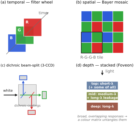
A bare sensor gives one number per photosite and color needs at least three, so the extra measurements must be borrowed from some other axis: time, space, depth, or a second piece of hardware. Whatever axis you spend, you usually lose the ability to discriminate along it. Multiplex in time and you must assume the scene holds still between frames; multiplex in space and you must assume color varies smoothly enough to interpolate the samples you skipped; multiplex in depth and you inherit badly overlapping bands you then have to un-mix. The only escape is to spend no scene axis at all and instead pay in hardware, with a beam-splitter and several sensors or an inverse-designed nanostructure, trading the assumption for cost and complexity. Each section below is one strategy: the technologies that use it, and the specific form this trade takes.
3.4.1 Multiplexing in time⧉
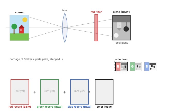
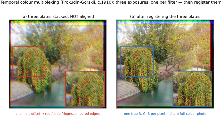
Shoot red, green, and blue frames sequentially through colored filters, or a rotating filter wheel. This is how Maxwell made the first color photograph (Maxwell 1861) and how Prokudin-Gorskii (Prokudin-Gorskii) captured the Russian Empire in three exposures. It is still how flatbed scanners, astronomy and fluorescence-microscopy filter wheels, telescope narrowband imaging, sequential-color machine-vision cameras, and many multispectral instruments work, because the same mechanism extends naturally from three filters to tens of narrow bands.
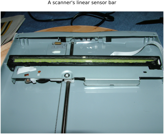
The implementations differ mainly in what does the sequencing. The oldest is a rotating filter wheel (or three separate plates) in front of a single sensor: three exposures through red, green, and blue filters, combined afterward. The first color photographs were made this way, Maxwell's 1861 tartan-ribbon demonstration and, half a century later, Prokudin-Gorskii's three-plate survey. Astrophotography still leans on it heavily: a cooled monochrome sensor (a mono sensor avoids the color filter array's light loss and keeps full resolution) sits behind a motorized filter wheel and stacks many long sub-exposures through each filter, red / green / blue for natural color or narrowband hydrogen, oxygen, and sulfur filters for nebulae, where nothing in the sky moves between frames. And every flatbed or document scanner is a time-multiplexer twice over: a sensor bar is swept mechanically down the page, which is itself how a one-dimensional line sensor becomes a two-dimensional image (scanning spends time to buy the spatial axis the sensor lacks), and color comes either from three passes under red, green, and blue illumination or from a tri-linear sensor with three colored rows. Field-sequential color television and some endoscopes ran the same spinning-color-wheel trick in real time.
The trade-off is discrimination in time: the method assumes the scene and camera hold still across the exposures. When they do, it is the best of every world, full spatial resolution, no demosaicking, no light split away, and as many bands as you care to spin past. When they do not, anything that moves between frames splits into colored fringes (Figure 3.4.6), and every temporal system must first register the plates to undo the small shifts between them (Figure 3.4.5), the simplest image-alignment problem in the book.
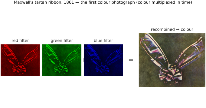
The three-color principle was demonstrated in 1861 by James Clerk Maxwell, the physicist who also unified electricity, magnetism, and light into the equations that bear his name. To show that any color can be matched by adding red, green, and blue, he had the photographer Thomas Sutton shoot a tartan ribbon three times through red, green, and blue liquid filters, then projected the three black-and-white positives back through the same three filters, superimposed, onto a screen. The overlap showed color: the first color photograph, and a live demonstration of trichromacy, the same three-number logic the rest of this book rests on. It very nearly should not have worked: the wet-collodion plates of the day were almost blind to red and green, and the "red" record came mostly from ultraviolet that the ribbon's red dye happened to reflect. A lucky accident, but the principle was exactly right, and every color camera since is a rearrangement of Maxwell's three filters. (Maxwell 1861)
3.4.2 Multiplexing in space: the color filter array⧉
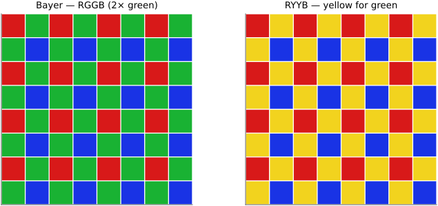
The dominant choice by far. Lay a color filter array (CFA) directly over the sensor so each photosite records one color and the missing two are filled in afterward by demosaicking (Figure 19). The archetype is the Bayer mosaic, two green photosites for each red and blue, its doubled green mirroring the eye's green-weighted luminance (the eye is itself a spatial CFA, its interleaved cone mosaic). The family is large: Fuji's X-Trans uses a less-periodic $6\times6$ tile whose irregularity scatters the moiré a strictly periodic grid produces, so it can drop the anti-aliasing filter; complementary CMY or CYGM (cyan-yellow-green-magenta) arrays pass more light through each filter than the primary RGB dyes; RGBW arrays add an unfiltered panchromatic "white" pixel for low-light sensitivity; and Huawei's RYYB swaps green for yellow to gather still more light.
The trade-off is discrimination in space: each pixel measures one color, so you must assume color varies smoothly enough that the two missing channels can be interpolated from neighbors. That assumption is usually safe, which is why the CFA won, but it costs a demosaicking guess (with false-color and zipper artifacts exactly where the assumption breaks), an optical low-pass filter to pre-empt those artifacts, some inter-channel crosstalk, and worst of all the roughly two-thirds of the light the absorptive filters throw away. Against those costs it is single-sensor, single-exposure, cheap, and motion-robust, which is why nearly every camera you own uses it.
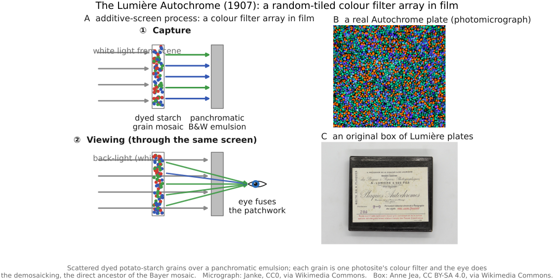
Color film reached the same spatial idea decades before silicon, by literally the same trick. The additive screen processes, the Lumière brothers' Autochrome (1907) and later Dufaycolor, Finlay, and Paget, coated the plate with a fine mosaic of transparent grains dyed red, green, and blue (Autochrome scattered dyed potato-starch grains at random; Dufaycolor printed a regular réseau grid) over a single panchromatic black-and-white emulsion. Each grain passed only its own color to the silver behind it, so the developed plate, viewed back through the same mosaic, rebuilt color from a spatial patchwork of filtered samples. This is a color filter array in film, the direct ancestor of the Bayer mosaic, random-tiled a full century early, with the dyed grain playing the photosite's role and the eye doing the demosaicking. (The other film tradition, the stacked-dye integral tripack of Kodachrome and modern color film, multiplexes color in depth instead, and so belongs with the Foveon below.)
3.4.3 Multiplexing across separate sensors: the beam-splitter⧉
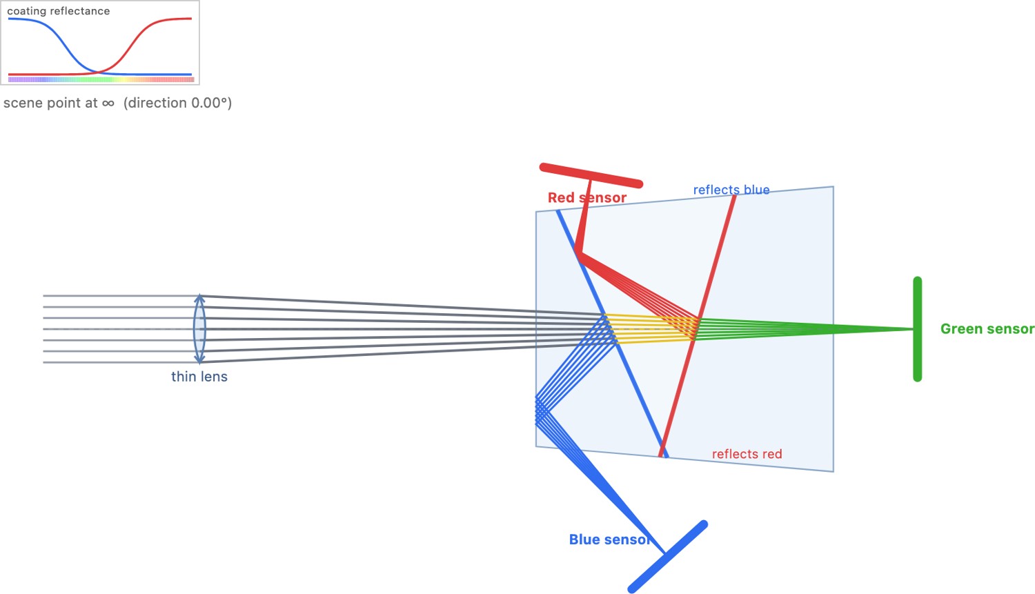
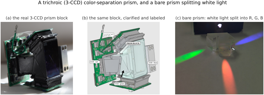
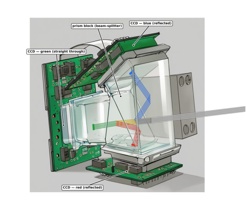
Send the whole image to more than one sensor and give each its own color. A dichroic prism block reflects each band onto its own chip (Figure 3.4.1c): the 3-CCD / 3-chip design long standard in broadcast video cameras, three-chip cinema and telecine cameras, and scientific and machine-vision multi-sensor rigs. Because the dichroic coatings split the light rather than absorb it, no photons are wasted and every channel keeps full resolution. (It is a dichroic beam-splitter, not a dispersing prism: it peels off three clean bands, it does not smear a spectrum.)
This strategy spends no scene axis, so it makes none of the constancy or smoothness assumptions of the other two: full resolution, full light, no demosaicking. Instead you pay the other currency, hardware complexity: three sensors registered to sub-pixel accuracy behind a bulky, expensive prism. That is why it never fit a phone or a cheap camera, stays confined to professional gear, and does not scale past a handful of bands.
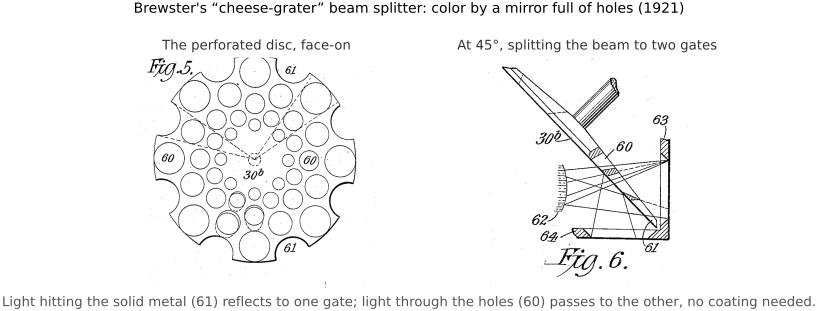
The hardware-splitting idea predates its dichroic form. Before interference coatings existed, P. D. Brewster's 1921 beam splitter divided a movie camera's beam with a polished metal disc drilled full of holes (Figure 3.4.9): light passing through the holes went straight to one color film gate, while light striking the solid metal between them reflected off to a second. It is the cheese-grater ancestor of the 3-CCD prism, the same bargain of spending hardware rather than a scene axis so that each color gets its own sensor. It was cruder in two ways: the fixed metal-to-hole ratio sets a single reflect/transmit split rather than a wavelength-selective peel, and because the disc splits by geometry and not by color, each path still needs its own color filter. So it lacks the dichroic prism's clean, lossless separation, but the core move is identical.
3.4.4 Multiplexing per pixel by dispersion: color routers and nano-prisms⧉
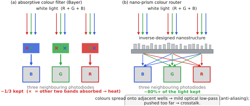
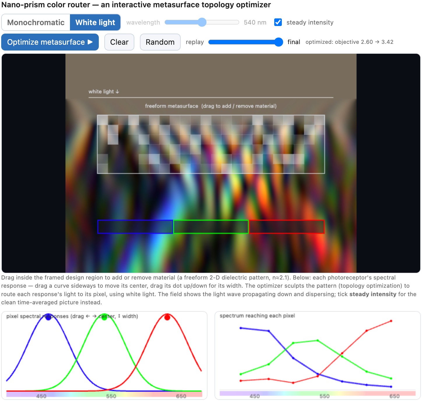
The Bayer mosaic and the 3-CCD prism sit at opposite extremes: Bayer multiplexes color across space but throws away two-thirds of the light to absorption; the prism splits light losslessly but needs three whole sensors. A color router (also called a color splitter or nano-prism) combines the two at the scale of a single pixel. In place of the absorptive filter it puts an inverse-designed nanostructure that acts as a tiny dispersing prism, redirecting each wavelength toward a different neighboring photodiode instead of absorbing it. So the color information is still multiplexed across space, Bayer-style, but achieved by dispersion rather than by masking, recovering most of the light the filters would have wasted (optical efficiency climbs from the filter's ~33% ceiling toward 80% and beyond, Nishiwaki et al. 2013; Zou et al. 2022). It is, almost literally, the broadcast prism shrunk to a per-pixel scale and laid flat on the sensor. The same per-pixel spreading has a second face: because each scene point's red, green, and blue are scattered onto different neighbors, a point's light is smeared across a small footprint, a built-in mild optical low-pass that doubles as the anti-aliasing the Bayer mosaic otherwise needs a separate filter for. Pushed too far, that smear becomes resolution-killing inter-pixel crosstalk, so the design game is to separate color cleanly while keeping the spread just wide enough to anti-alias and no wider. The idea runs from Panasonic's 2013 color splitters to inverse-designed metasurface routers; the first shipping cousin, Samsung's "Nanoprism," takes the gentler step of replacing only the microlens to funnel light into the color filters it keeps. (See also the sensor-tricks section, where the nano-prism appears as a light-efficiency trick.)
The trade-off, then, keeps the CFA's spatial smoothness assumption and its reconstruction step, but swaps the filter's light loss for fabrication complexity: the routers are inverse-designed and hard to make, and pushed too far the dispersion becomes crosstalk.
3.4.5 Multiplexing per pixel by tunable absorbers: quantum dots⧉
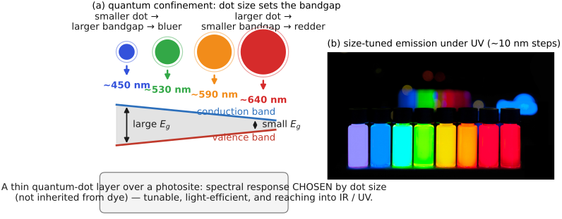
A newer material sits as a hybrid of the spatial mask and the prism idea. Colloidal quantum dots (semiconductor nanocrystals whose absorbed wavelength is set by their size through quantum confinement) can be laid down as a thin, per-pixel light-absorbing layer whose spectral response is chosen rather than inherited from dye chemistry. Like the spatial CFA, they place a color-selective element over each photosite (color is still multiplexed across space); but like the prism / dispersion route, they can be engineered (tuned narrower or sharper, and paired with dispersive routing) to stop discarding the two-thirds of the light an absorptive dye filter throws away, while also reaching into the infrared and ultraviolet that silicon handles poorly and absorbing in far less depth (a boon for the sub-micron pixels of the sensors chapter). They point past the fixed Bayer settlement toward a sensor whose very spectral sensitivities are a design parameter (developed as such in the spectral-sensitivity section below). The trade-off is again spatial, so demosaicking stays, and the win in tunability and efficiency is paid for in the maturity of a newer material, with its own noise and stability questions still being worked out.
3.4.6 Multiplexing in depth: stacked photodiodes⧉
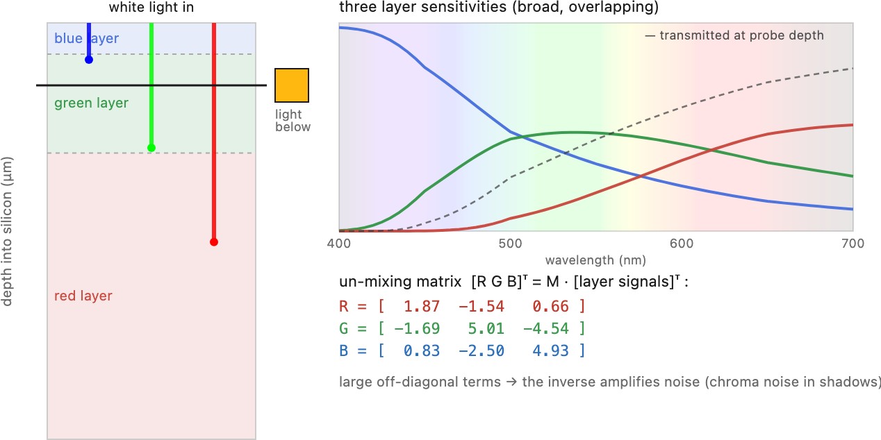
Avoid color filters entirely and exploit the fact that silicon itself absorbs light by depth: short (blue) wavelengths within the first micron or so, green deeper, red deepest of all. Stack three photodiodes at different depths in the same silicon and each collects a different slice of the spectrum: the Foveon sensor (in Sigma cameras), conceptually like Kodachrome's stacked dye layers. Because all three layers sit at the same location, it captures color at every pixel with no demosaicking and no CFA. A common simplification hides an important detail: the layers are not red, green, and blue at three depths. Absorption is gradual and cumulative: the top layer catches blue plus a good deal of everything else passing through on its way down, the middle catches green plus leaked red, the bottom catches whatever is left, so the three layer responses are broad and heavily overlapping, nothing like clean primaries (Figure 3.4.1d). Recovering RGB therefore means multiplying the raw layer signals by a color matrix, and because the responses overlap so much, that matrix is ill-conditioned: it has large off-diagonal terms and amplifies noise as it inverts the overlap, which is exactly why Foveon images are prized for crisp luminance detail yet are noticeably noisier in chroma, especially in the shadows. (Overlapping sensitivities that need an ill-conditioned un-mixing are a recurring headache, the very same one the eye's own overlapping L and M cones cause, the non-orthogonality lesson of the previous chapter.)
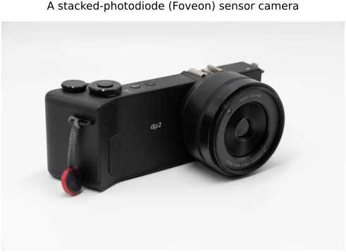
Few production cameras have ever used a Foveon sensor; the Sigma dp series is the best known (Figure 3.4.16), sold on exactly the trade above: unusually crisp, demosaicking-free luminance detail in exchange for noisier color, a modest ISO ceiling, and slow readout.
Quantitatively (Figure 3.4.17), silicon's absorption length climbs steeply with wavelength: blue light around 450 nm is mostly absorbed within roughly half a micron, green around 550 nm takes a couple of microns, and red around 610 nm penetrates several microns before it is caught. Stacking the three photodiodes across those depth bands yields sensitivities that are not three tidy bumps but three broad, sagging curves with enormous overlap: the top (blue) layer collects a large share of green and red on their way through, and so on down. The matrix that inverts these layer signals back to RGB is correspondingly ugly, with off-diagonal terms as large as the diagonal and of opposite sign, so a little read noise in one layer is multiplied severalfold into the recovered chroma. That is the concrete cost of spending no spatial or temporal axis: the color lives entirely in small differences between heavily overlapping depth signals, and small differences of noisy numbers are noisy.
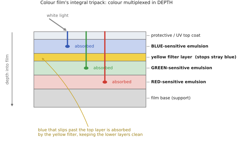
Depth multiplexing is not a silicon invention; color film got there first, chemically. The dominant color-film design, the integral tripack of Kodachrome, Ektachrome, and every C-41 negative, stacks three light-sensitive emulsion layers on one base: a blue-sensitive layer on top, then a green-sensitive layer, then a red-sensitive layer, with a thin yellow filter layer just below the top one to stop stray blue (to which all silver halides respond) from leaking into the lower layers. White light enters the top and is caught band-by-band with depth, exactly the Foveon idea, and after development each layer forms its own complementary dye so the stack yields full color at every point with no spatial mosaic (Figure 3.4.18). It is the same trade the Foveon makes and the same one the Autochrome does not: color multiplexed in depth (stacked, full-resolution, no demosaicking) rather than across space (a mosaic that must be interpolated). Silicon's Foveon is the integral tripack rebuilt in a semiconductor, absorption depth standing in for the sensitized layers.
3.4.7 Hybrid strategies⧉
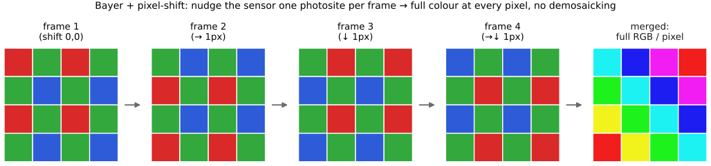
Real cameras often combine strategies, and the most useful hybrid is Bayer plus pixel-shift (Figure 3.4.19). A piezo actuator nudges the sensor by exactly one photosite between frames, so that over four exposures every output location is sampled through a red, a blue, and both green filters in turn; merge the four and you get true R, G, B at every pixel with no demosaicking guesswork (full color resolution and much lower noise) at the cost of needing a static scene on a tripod. (It is the spatial Bayer trick borrowing the temporal axis to fill its own holes.) Shift by half a photosite instead and you reach past the sensor's nominal resolution: a multi-frame super-resolution. Video pipelines hybridise the other way, leaning on motion across frames; astrophotography filter wheels are temporal multiplexing with cooled sensors. The strategies are a toolkit, not a fixed menu.
3.4.8 Beyond trichromatic capture: full spectrum and multispectral⧉
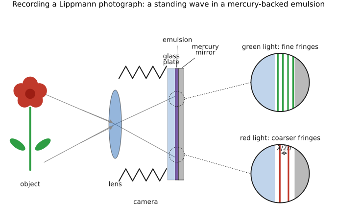
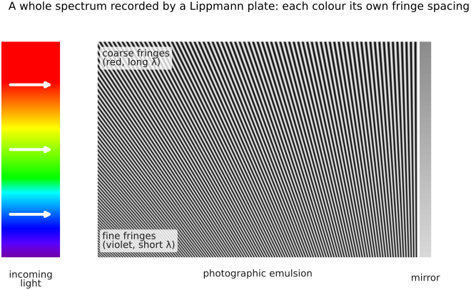
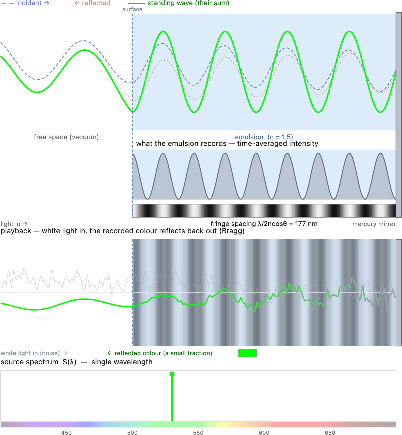
One method stands apart by refusing the three-number compromise altogether. Lippmann photography (Lippmann colour photography (Alternative Photography); Bjelkhagen, "Lippmann photography") records the full spectrum at every point as a physical interference pattern recorded along the depth of the film (Figure 3.4.20). The depth dimension does not record the light spectrum directly but an interference pattern instead. Light passes through a fine-grain transparent emulsion backed by a mirror of liquid mercury, so the incident and reflected waves superpose and form interference patterns in a manner similar to thin-film interference, the same physics that tints a soap bubble and the anti-reflection coating on a lens (thin-film interference and structural color, §2.1).
First consider a monochromatic wave with wavelength $\lambda$. Its reflection and it interfere into a standing wave whose antinodes are spaced by $\lambda/2$ and which gets recorded by the emulsion, forming a kind of filter. Later, viewed in white light, the recorded pattern act as a so-called Bragg reflector and send back exactly the wavelengths that made them by filtering the white light and keeping only the recorded wavelength.
Similar effects occur with a more complete spectrum where the incoming light and its reflection form an interference patterns than gets recorded and then acts as a filter for white light to reproduce the incoming spectrum. The plate stores true spectral information, not a trichromatic projection (the limiting case of color capture), which won Gabriel Lippmann the 1908 Nobel Prize (Lippmann 1891) and prefigured holography. Modern signal-processing analysis has even recovered the original spectra from surviving 19th-century Lippmann plates (Baechler et al. 2021), confirming that the full spectral information really is physically preserved. It never became practical (exposures of minutes, awkward viewing), but it is the conceptual endpoint: every other sensor on this page is a lossy three-number approximation of what Lippmann captured in full.
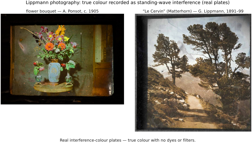
Gabriel Lippmann (1845–1921) won the 1908 Nobel Prize in Physics "for his method of reproducing colors photographically based on the phenomenon of interference", the only Nobel ever awarded for a color-photography process, and one almost nobody ever used. He was a physicist's physicist: he also built the capillary electrometer (which recorded the first electrocardiograms), worked on piezoelectricity alongside the Curies, and proposed integral photography, the lenticular ancestor of today's light-field cameras. His color plates are physically gorgeous and maddeningly impractical (minute-long exposures, a sheet of liquid mercury pressed against the emulsion, and an image you can only see from the right angle), yet they remain the only photographs that store the actual spectrum of a scene rather than three numbers per point. A standing reminder that the trichromatic shortcut every other sensor on this page takes is a choice, not a law of nature.
3.4.9 Spectral sensitivity: matching the eye, catching photons, and white balance⧉
The exact shape of a color sensor's three spectral-sensitivity curves (the $r(\lambda)$ of the red, green, and blue channels, built earlier by the color-filter array on the photosites of Sensors: photosites, CCD vs CMOS) is one of the camera's most constrained choices, because it is pulled in three directions at once that cannot all be satisfied.
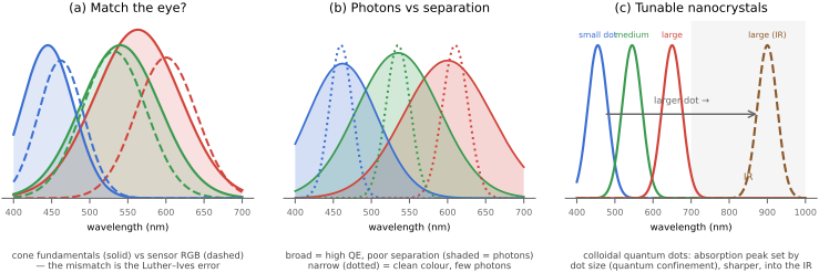
- Fidelity to human vision. For a camera to record the color a human would see, its three curves should be a fixed linear combination of the eye's cone fundamentals (equivalently, of the CIE color-matching functions), the Luther–Ives condition. A sensor that met it could be mapped to human color by a single $3\times3$ matrix with no error. Every real sensor violates it, because silicon-plus-dye curves are simply the wrong shape, and the penalty is a metameric error no color matrix can remove: two spectra that look identical to the eye read as different RGB, and two that look different can read the same. The color-correction matrix in the ISP is a least-squares compromise: right on average, wrong on the hard cases (saturated reds, narrow-band LEDs, foliage).
- Quantum efficiency and noise. Quantum efficiency (the fraction of arriving photons actually counted) rewards broad, overlapping passbands: the wider each filter, the more photons reach the well and the higher the SNR. But broad overlap is exactly what destroys color separation, because strongly correlated channels must be differenced to pull color out, and differencing amplifies noise (the same reason the eye's overlapping L and M cones force an opponent stage, L2.14). Narrow, well-separated filters give clean color but throw photons away and read noisier. The green-doubled Bayer is one point on this curve: spend photons and resolution where the eye cares most (luminance), economize on chroma.
- White balance across illuminants. Because each channel integrates illuminant × reflectance × sensitivity, changing the light changes the raw RGB of a fixed object. Undoing that, white balance, ideally a per-channel gain (von Kries), is only exact when the sensitivities behave like the cones; the further they stray, the more a single diagonal (or even $3\times3$) fails to hold colors constant as the light shifts from daylight to tungsten to a spiky fluorescent. Good spectral design makes white balance more reliable across illuminants (→ auto white balance).
These three pull against each other: the curves that best match the eye are broad and overlapping (bad for separation), the curves that separate color cleanly are narrow (bad for QE and for matching the eye), and keeping white balance stable across odd illuminants wants yet another shape. Every color sensor is a negotiated settlement among them (Figure 3.4.24).
Recap: big lessons of this chapter
Strip away the color filter and a sensor is monochrome at the pixel: each photosite reports a single number, the count of photons it caught — not a color. The three (or more) values that color needs must therefore be multiplexed along some other axis: over space (a color-filter array such as Bayer, paying with resolution and a demosaicking step), over time (sequential color filters, paying with motion robustness — the old color-wheel and many scientific cameras), across multiple sensors (a beam-splitter prism feeding three chips, the 3-CCD video camera, paying with bulk and cost), or over depth (wavelength-dependent absorption in stacked photodiodes, the Foveon, paying with noise). Every color camera is a choice of which axis to spend. The same constraint shapes the eye, whose three cone types sample color over space at the retina (L2.10, L2.13).